D-Orbital Geometry - Part 2

Introduction

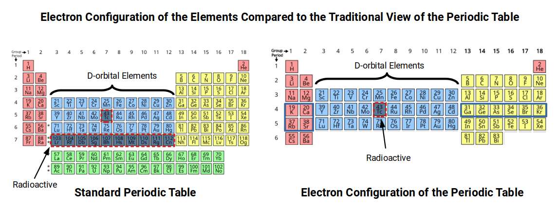
The 2nd D-orbital set spans elements 39 to 48 on the periodic table — from Yttrium to Cadmium. In standard quantum theory, this row is notable chiefly for being anomalous: more elements in this set break the Aufbau Principle than follow it, Technetium (43) is the only naturally radioactive element among the stable elements without a plausible nuclear reason, and Silver (47) is the most electrically conductive element in the periodic table by a margin that quantum mechanics cannot explain from first principles.

The geometric model of Atomic Geometry resolves all three mysteries with a single underlying cause. The 1st D-orbital set (elements 21–30), covered in D-orbital Geometry Part 1, is governed by the Rhombic Cuboctahedron — the template for 4D hypercubic space. The 2nd D-orbital set is governed by the Truncated Cube, which orientates two Rhombic Cuboctahedra through the Silver Ratio and produces the template for 5D hypercubic space. This dimensional step-up is not a metaphor: it is encoded directly in the geometry of the electron cloud, and it is what causes every anomaly in the set.

Technetium (43) sits at the exact midpoint of the three stable D-orbital sets, where two Tesseract cells share a middle cube in the 5D shadow projection — a position of inherent geometric instability. The Aufbau anomalies of Niobium (41) and Molybdenum (42) arise because the Truncated Cube structure demands a precise lobe count to maintain balance, overriding the simple energy-filling rule. And Silver (47) is the most conductive element because its radius is exactly the Golden Ratio (1.618Å), placing its Tetrakis Octahedron geometry in perfect resonance with the Brillouin Zone lattice at multiple scales.

This article builds directly on Part 1. It begins with the seven geometric principles that underpin Atomic Geometry, then traces the transition from 4D to 5D geometry as the 2nd D-orbital set forms. From there it works through the set element by element, showing how each radius, each anomaly, and each exceptional property emerges as a natural consequence of the geometry. Part 3 will build on this foundation to examine the 3rd D-orbital set and the transition into 6D hypercubic space.

Problems with Quantum Theory

Before examining the 2nd D-orbital set, it is worth reviewing what the geometric model resolves within present quantum theory — because the anomalies in this set expose the limits of the standard approach more clearly than any other row of the periodic table.

In our examination of the P-orbital elements, we highlighted that many elements in each set exhibit the same radius. In the 2nd P-orbital set, Phosphorus (15), Sulphur (16), and Chlorine (17) all exhibit an experimentally determined radius of 1Å. In the 3rd P-orbital set, Arsenic (33), Selenium (34), and Bromine (35) all have a radius of 1.15Å — appearing in exactly the same groups (15, 16, and 17). A similar pattern holds across D- and F-orbitals: apart from the first element of each D-orbital set, the others all cluster at 1.4Å or 1.35Å. F-orbital elements settle near 1.75Å for the first half of the set. This uniformity is traditionally attributed to F and D block contraction — electron shielding reducing the effective nuclear charge. Yet no rigorous mathematical derivation of this contraction exists, and it cannot account for the uniform radii in P-orbitals, which appear before any D- or F-orbitals form.

The standard model also predicts a continuously shrinking radius as the nucleus grows — yet this is not observed. In the 2nd D-orbital set, the radius of Palladium (46) is larger than that of Rhodium (45), and Silver (47) is larger still. Standard theory has no geometric explanation for this.

According to quantum mechanics, it offers highly accurate predictions for the atom. In practice, this accuracy applies only to 'hydrogen-like' atoms, and even there it breaks down: the experimentally determined radius of hydrogen is 0.25Å, yet the Bohr model predicts 0.53Å — an error of over 100%. Published sources typically present the theoretical prediction rather than the experimental value; only by consulting the underlying datasets is this discrepancy visible.

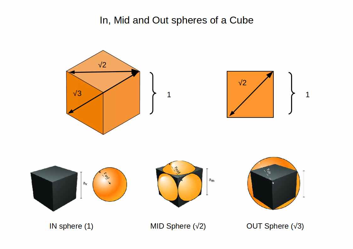
Seen through the lens of geometry, a clear pattern emerges from the radii data. From 0.25Å for Hydrogen (1), the P-orbital sets double: 0.5Å, then 1Å. The 3rd P-orbitals settle at 1.15Å — the difference between the 2nd and 3rd P-orbital radii corresponding to the difference between the out-sphere and mid-sphere of a Rhombic Dodecahedron. The 4th P-orbitals reach approximately √2 ≈ 1.4Å, matching the D-orbitals. The F-orbitals settle near 1.75Å, close to √3. The ratios 1, √2, and √3 are the in-, mid-, and out-sphere of a cube with a side length of 2. This is not coincidence: it is the geometric skeleton of the periodic table.

One further contradiction in quantum mechanics deserves attention. The Schrödinger equations are widely described as wave equations predicting the probability of finding an electron at a given location — but they are more accurately heat equations, describing flow from one state to the next. Since the atom is quantised into discrete bands, this flow cannot be continuous. Standard interpretations oscillate between describing electrons as having a probability of being anywhere and constraining them to specific quantised energy levels. The contradiction arises from insisting on treating the electron as a particle.

The wave nature of electrons was first proposed by Louis de Broglie in 1924 and confirmed by the Davisson–Germer experiment. De Broglie's insight led Erwin Schrödinger to develop his equations, which were later adapted to include quantised spin. The notion of wave–particle duality stems from the inability of the standard model to resolve the Ultraviolet catastrophe and Photoelectric effect without reintroducing the particle nature of light.

The theory of Atomic Geometry proposes that the Schrödinger equations depict the transformation of one geometric solid into another, producing the quantised states described by quantum mechanics. With each progressive element, the geometry of the nucleus and electron cloud changes shape, producing the variation in atomic radii and quantising the electron cloud into discrete bands through the in-, mid-, and out-sphere of each solid. This approach resolves wave–particle duality, probability theory, and quantum entanglement simultaneously — replacing them with a logical, consistent geometric description — and reintroduces the concept of the Aether as a 4D geometric medium. Quantised spin values are explained as the rotation of 4D and higher-dimensional polytopes forming the boundaries of atomic structure.

The Atomic Geometry model already provides a close approximation of the electron cloud without heavy parameter fitting. A more detailed picture, including conductive and magnetic properties, is examined in the article on Brillouin Zones.

Geometric Principles

The theory of Atomic Geometry is predicated on seven geometric principles. Understanding these principles is essential for following the analysis in the remainder of this article.

1. In-, Mid-, and Out-spheres. Any 3D solid produces three concentric spheres. For a cube, the in-sphere touches the centre of each face, the mid-sphere passes through the midpoint of each edge, and the out-sphere touches each corner. This produces the quantisation of the electron cloud: the reason electrons occupy discrete energy bands is this geometric fact. The Schrödinger probability transformations are a consequence of it.

2. The Jitterbug. Originally popularised by Buckminster Fuller, the Jitterbug Construction describes a transformation sequence between related solids. Fuller included three forms: the Octahedron, Icosahedron, and Cuboctahedron. Atomic Geometry adds two more — the Snub Cube and the Rhombic Cuboctahedron — producing the Extended Jitterbug.

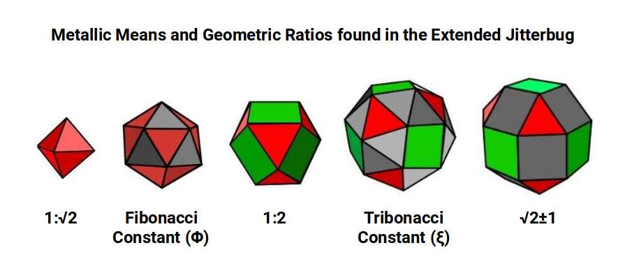
These solids transform from one to the next by progressively opening the triangular faces of the Octahedron. The Icosahedron forms when two triangles appear in each gap; the Cuboctahedron when square faces emerge. The Snub Cube and Rhombic Cuboctahedron continue this expansion. The Cuboctahedron is the only solid whose side length equals its radius, making it ideal for nesting 13 spheres in hexagonal close-packing.

The sequence can also be inverted, indicative of a 4D polytope and corresponding to the quantised UP/DOWN spin of the electron. A more accurate description is the rotation of the 4D hypercube on its w-axis, which produces quantised ½-integer spin values, as described in the article on the 4D Electron Cloud.

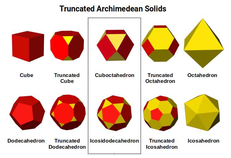
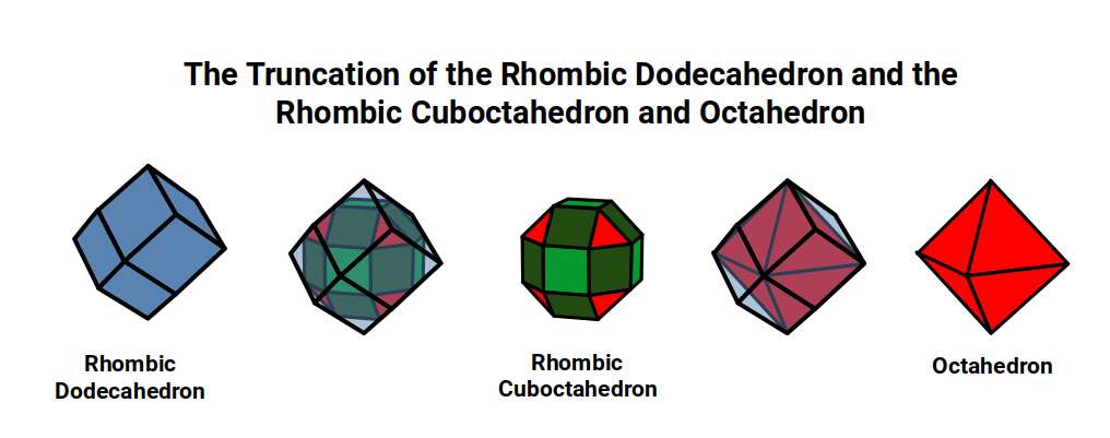
3. Truncation. Removing the corners of a solid at the halfway or one-third point of each edge produces a new solid. The Cuboctahedron is produced by truncating a Cube or Octahedron at its halfway point. Truncation generates 7 of the 13 Archimedean solids.

4. Explosion. When the faces of a solid are moved outward from the centre, new faces appear in the gaps. The Rhombic Cuboctahedron is produced by exploding a Cube or Octahedron: its 8 triangular faces derive from the Octahedron, and 6 of its square faces from the Cube.

5. Duality. Dual solids share the same number of corners as the other's faces. An Octahedron can be placed inside a Cube so that its corners define the centre of each face, and vice versa. The Cube and Octahedron are duals; so too are the Dodecahedron and Icosahedron.

6. Nesting. Solids can be nested concentrically. Not all nested pairs are formed from duals — for example, a Cube can be nested inside a Dodecahedron in up to five distinct orientations, which is central to the 5D hypercube model discussed below.

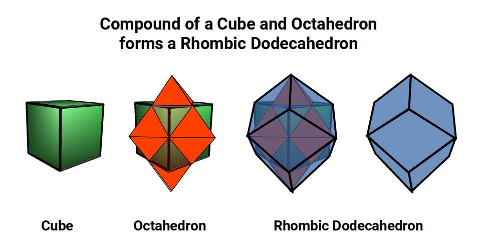
7. Compounds. Two solids can be positioned so that their mid-spheres are aligned. When the Cube and Octahedron are compounded in this way, removing the corner caps produces a Cuboctahedron (the 'hull' of the compound), while connecting the corner points produces a Rhombic Dodecahedron. The Rhombic Dodecahedron is the template for the 4D hypercube (tesseract).

These seven principles produce logical geometric transformations that show how one solid transforms into the next, providing a purely spatial description of what the Schrödinger equations depict probabilistically. Through them, we can build a geometric blueprint that explains how space evolves from the 5 Platonic Solids into 4D, 5D, 6D, and higher-dimensional polytopes.

From 4D to 5D: The Dimensional Step Between the D-Orbital Sets

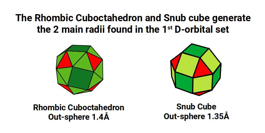
The geometric principles above underpin the structure of all orbital types. For S-orbitals and P-orbitals the governing forms are a Sphere and Octahedron respectively. The 1st D-orbital set is governed by the 4D Rhombic Cuboctahedral model: a cube with a side of 1 explodes to form the Rhombic Cuboctahedron with an out-sphere of 1.4Å, which then collapses through the Jitterbug into the Snub Cube with an out-sphere of 1.35Å, generating the two main radii of the 1st D-orbital set.

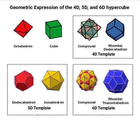
This 4D model is built from the compound of a Cube and Octahedron, which produces the Rhombic Dodecahedron — the geometric template for the 4D hypercube (Tesseract). The natural question is: what comes next? What is the template for 5D hypercubic space?

The answer begins with the Dodecahedron. A Cube can be nested inside a Dodecahedron in 5 distinct orientations, with the edges of all five cubes tracing a pentagram across each dodecahedral face. We propose that this nesting structure is the template for the 5D hypercube — an observation not presently recognised in modern geometry.

The Dodecahedron can also be nested around a Cube in two distinct orientations, analogously to the star-tetrahedron nested in a Cube. Eight of the Dodecahedron's 20 corners define the corners of the Cube, with the remaining 12 corners falling in 6 pairs above each face.

The Cube can also be rotated through four 90° orientations on its north–south axis, bringing the total number of Cube orientations within the Dodecahedron to 40 — equal to the number of cubic faces forming a 5D hypercube. Each of these 4 rotations can be understood as a single Tesseract cell, of which 10 make up the faces of the 5D cube.

The 5D cube has 32 corners (2⁵) — the combined corner count of a Dodecahedron and Icosahedron. When these dual solids are compounded, their corners connect to form the Rhombic Triacontahedron — the template for the 6D hypercube, in the same way the Rhombic Dodecahedron is for the 4D hypercube. This establishes a clean geometric sequence: the 3D cube compounded with the Octahedron produces 4D; nested in the Dodecahedron it produces 5D; compounded with the Icosahedron it produces 6D.

The 5D cube can be depicted as a shadow projection of 3 nested cubes — a middle cube shared between two Tesseract cells. Analogously, a 4D cube projects as one cube nested inside another, and the 6D cube as 4 nested cubes. We also propose that the 5D shadow can be represented by replacing the two outer cubes with Rhombic Dodecahedra, with the middle cube shared between the two Tesseracts.

With the 4D–5D–6D sequence established, we can now show precisely how the 2nd D-orbital set embodies this 5D template — and why that single geometric fact explains every anomaly in the set.

The Truncated Cube: Geometric Model of the 2nd D-Orbital Set

In Atomic Geometry, the 1st D-orbital set is modelled by a Cube with a side of 1 that explodes to form the Rhombic Cuboctahedron. A second Cube with a side of √2 nests inside, with its corners centred on the triangular faces of the Rhombic Cuboctahedron. This larger cube can be truncated to produce a Cuboctahedron with a side of 1. Similar to the Rhombic Dodecahedron, this nested structure also models a 4D hypercube. The wire frame of the Rhombic Dodecahedron, viewed from above, produces the shadow projection of this geometric construct.

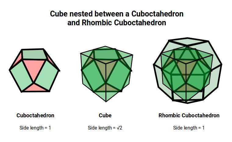
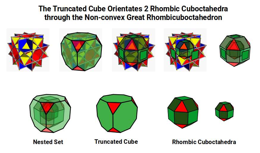
The 2nd D-orbital set builds on this by replacing the Rhombic Cuboctahedron with the Truncated Cube. Both forms exhibit an octagon: in the Rhombic Cuboctahedron it appears as a rotatable midsection; in the Truncated Cube it appears on each of the six faces derived from the Cube. The octagon encodes the Silver Ratio (√2 ± 1) — and this encoding is precisely what marks the step from 4D to 5D geometry.

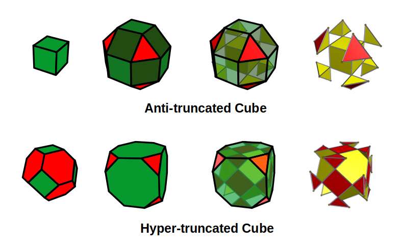
By removing the square faces of the Rhombic Cuboctahedron, a Cube is revealed at its centre, with 8 sets of tetrahedral solids at each corner in a ratio of 1:√2 — forming the Anti-Truncated Cube. A similar operation applied to the Truncated Cube generates the Hyper-Truncated Cube, whose interior resembles a Truncated Octahedron with hexagonal faces in a ratio of 1:√2.

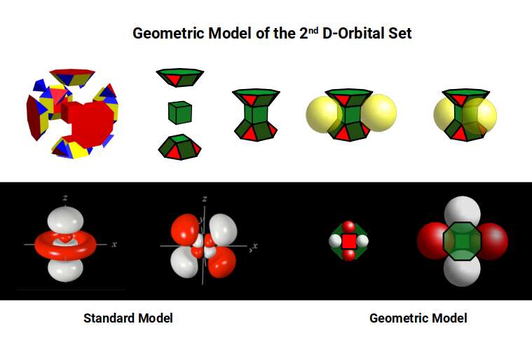
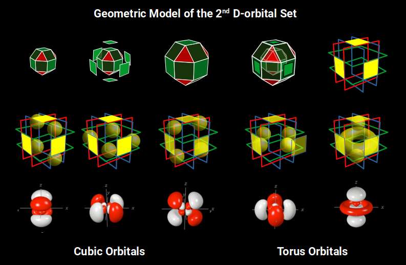
The Rhombic Cuboctahedron divides into three sections — a central octagonal prism that rotates in 45° steps between fixed top and bottom sections. In the 1st D-orbital model, this rotation explains the 5th torus orbital. In the Truncated Cube, the top and bottom sections are inverted so that their square faces touch those of the central Cube. This produces a central column lying at the centre of a torus field, with 4 adjacent spaces on each face of the cube forming cross-shaped patterns when viewed from above — directly corresponding to the 4 D-orbital lobe types.

The Truncated Cube can also be defined by 16 interlocking squares forming the 'Non-convex Great Rhombic Cuboctahedron'. This form contains two nested Rhombic Cuboctahedra at different scales: if the larger has a side of 1, the smaller has a side of √0.5 (= √2 ÷ 2). When the square faces of the inner form are projected outward, each falls inside the 8-pointed star on each face of the non-convex polyhedron. This relationship expresses the Silver Ratio as √0.5 ± ½.

In this way, the Truncated Cube orientates two Rhombic Cuboctahedra. Whereas a single Rhombic Cuboctahedron produces a model of 4D cubic space, two combined produce the template for 5D cubic space, mediated by the Silver Ratio. This is the key structural difference between the 1st and 2nd D-orbital sets.

The non-convex form consists of 16 square planes: 6 in horizontal/vertical orientations, and 10 along the diagonals. The 6 vertical planes divide a cube of space into 27 small parts (3³). With the corners removed for the Truncated Cube, this reduces to 19. A complete D-orbital set has 5 orbital types; counting the torus shape as a single lobe gives 18 + 1 = 19 total — matching the number of cubic spaces exactly.

Of these 19 spaces, only those in the central planes are uniform cubes (the octagonal faces of the Truncated Cube distort the others). This is where the torus D-orbital and one of the rotated cross D-orbitals are located. In Atomic Geometry these are termed the 2 Torus Orbitals, falling in the same orientation as the P-orbital sets, while the remaining 3 are termed Cubic Orbitals, as they define the midpoints of the sides of a Cube.

A Rhombic Dodecahedron is composed of a compound of a Cube and Octahedron. In the structure of the electron cloud, the 3rd P-orbital set forms over a completed 1st D-orbital set and is represented by this compound — the template for 4D hypercubic space. This explains why the 3rd P-orbital radii settle at 1.154Å rather than continuing the doubling pattern: the difference between the 2nd P-orbital radius (1Å) and the 3rd (1.154Å) corresponds to the difference between the mid-sphere and out-sphere of the Rhombic Dodecahedron.

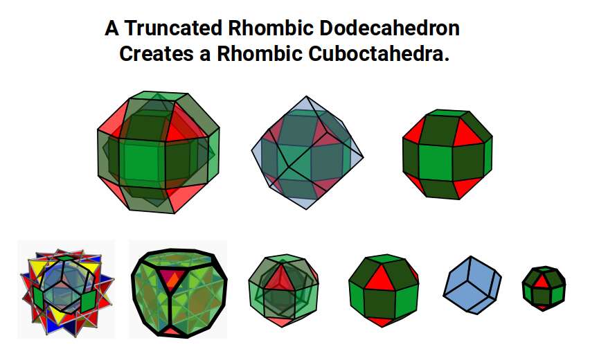
In Atomic Geometry, the 1st D-orbital set is represented as a Rhombic Cuboctahedron created by truncating a Rhombic Dodecahedron. The 2nd D-orbital set produces a second Rhombic Cuboctahedron whose size and spacing are defined by the Non-convex Great Rhombic Cuboctahedron, generated by the Truncated Cube. A Rhombic Dodecahedron placed around the smaller Rhombic Cuboctahedron — so that its outermost corners touch the centre face of the larger — completes the relationship between the two scales. The combination of the Truncated Cube and Rhombic Dodecahedron therefore produces what we consider the template for 5D Hypercubic space.

Transition from the 1st to the 2nd D-Orbital Set

Having established the geometric template, we can now trace the exact path by which the atomic structure transitions from the completed 1st D-orbital set into the 2nd. This transition is itself geometrically determined — and it defines the starting radii of the new set.

After the 1st D-orbitals complete in the 3rd electron shell (elements 21–30), a 3rd set of P-orbitals (elements 31–36) starts to form in the 4th shell. After Potassium (19) and Calcium (20) form in the 4th shell, the 1st D-orbitals fill the 3rd shell below. Once complete, elements 31–36 fill the 4th shell as P-orbitals. The pattern then repeats: two S-orbital elements, Rubidium (37) and Strontium (38), form in the 5th shell before the 2nd D-orbital set completes in the 4th shell below.

After the 1st D-orbitals complete with a radius of 1.35Å, the P-orbitals that follow progressively shrink until Arsenic (33), Selenium (34), and Bromine (35) all exhibit the same radius of 1.154Å — again contradicting the standard model's prediction of a continuously shrinking radius. Atomic Geometry explains this: the radii of the 2nd and 3rd P-orbitals correspond to the out-sphere and mid-sphere of the Cuboctahedron (or more accurately the Rhombic Dodecahedron), and the Octahedron contained within the Rhombic Dodecahedron can also be reproduced by truncating its corners.

S-orbital elements generally exhibit a much larger radius. Rubidium (37) has a radius of 2.35Å (more than double the preceding P-orbitals), followed by Strontium (38) at 2Å.

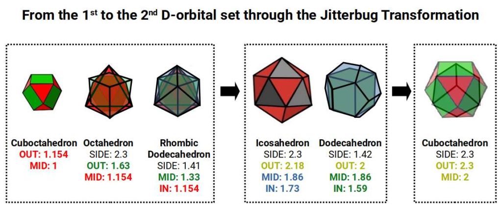
The Cuboctahedron with a side of 1.154Å has a mid-sphere of 1Å, matching the 2nd and 3rd P-orbital radii. Its dual, the Rhombic Dodecahedron, is composed of a compound of an Octahedron and Cube. The Octahedron has a side of approximately 2.3Å (= 4÷√3), producing an out-sphere of 1.63Å. The Cube has the same side length and an out-sphere of √2 = 1.41Å. The mid-sphere of the Rhombic Dodecahedron is 1.33Å. Together, these three radii — 1.63Å, 1.41Å, and 1.33Å — provide an extremely close match to the three types of radius found in the 1st D-orbital set.

The Octahedron can transform into a Cuboctahedron through the Jitterbug, producing a larger out-sphere of 2.3Å (matching Rubidium (37)) and an in-sphere of 2Å (matching Strontium (38)). The Icosahedron, which forms in the transition between these two, has an out-sphere of 2.18Å and an in-sphere of 1.86Å — matching the preceding S-orbitals Potassium (19) and Calcium (20). This single geometric model therefore maps all radii from element 19 through to element 38. The full derivation is given in D-orbital Geometry Part 1.

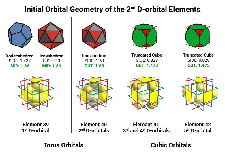
Similarly, the Icosahedron and Dodecahedron can be compounded (by aligning their mid-spheres at 1.86Å). This radius matches both Calcium (20) and the first element of the 2nd D-orbital set, Yttrium (39). When compounded, the Dodecahedron exhibits an out-sphere of 2Å (matching Strontium (38) and the Cuboctahedron mid-sphere), a mid-sphere of 1.86Å, and an in-sphere of 1.59Å — closely matching Yttrium (39) and Zirconium (40). In this way all elements from Phosphorus (15) through Zirconium (40), and all but one of the F-orbital elements, are geometrically defined.

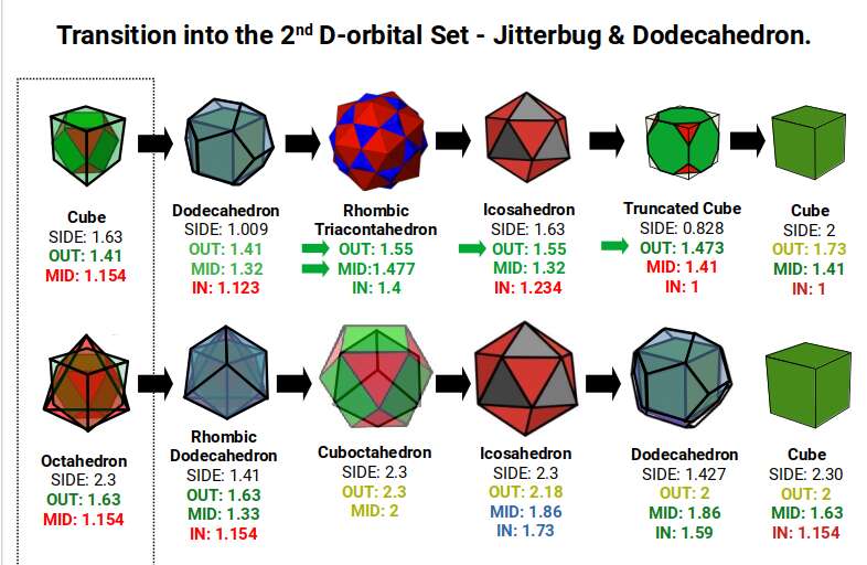
As the Rhombic Dodecahedron is produced from the compound of an Octahedron and Cube (formed by the completed 1st D-orbital set and 3rd P-orbitals below), another geometric transformation becomes possible. The Cube nested around the Cuboctahedron can be placed inside a Dodecahedron, both sharing an out-sphere of 2Å. The mid-sphere of the Cube will be 1.154Å (average of the 3rd P-orbital set), and the mid-sphere of the Dodecahedron 1.32Å. When compounded with an Icosahedron to form the Rhombic Triacontahedron (template for 6D hypercubic space), this produces an out-sphere of 1.55Å — the radius of Zirconium (40).

The Rhombic Triacontahedron has a mid-sphere of 1.47Å, which is the radius of Niobium (41) and Molybdenum (42), and is only fractionally larger than the out-sphere of the Truncated Cube derived from a Cube with side length 2.

The preceding S-orbitals appear in the 5th shell with radii of 2.3Å and 2Å — both present in the Jitterbug transformation. When the first D-orbital element, Yttrium (39), forms, the radius contracts to 1.85Å (the mid-sphere of the Icosahedron–Dodecahedron compound). This is the 1st torus orbital type. With Zirconium (40), the torus orbital set completes, and the radius contracts into the smaller Icosahedron.

After this, the pattern would normally produce a radius of 1.32Å (mid-sphere of the Dodecahedron), but because the torus is already complete, the Cubic D-orbitals begin to form instead, changing the structure to a Truncated Cube. At this point Niobium (41) transforms one of its S-orbital electrons into an additional D-orbital electron — the first of the Aufbau anomalies discussed in the next section. The Truncated Cube is sustained by producing 4 orbital lobes above the torus ring and 4 below. Molybdenum (42) then completes the D-orbital half-set.

The Atomic Geometry model consistently falls within the experimentally determined margin of error of ±5Å for the radii of these elements. The Bohr model in most cases predicts a much larger radius — a discrepancy traditionally attributed to D-block contraction, for which no rigorous mathematical derivation exists.

As the first two 2nd D-orbital elements are found in the out-sphere and mid-sphere of the Dodecahedron — which we propose forms the blueprint of 5D Hypercubic space — the 2nd D-orbital set begins to construct a 3rd Cube, indicative of the shadow projection of a 5D hypercube: 3 nested cubes, or 2 nested Tesseracts sharing a middle cube.

The Aufbau Anomalies: Niobium (41) and Molybdenum (42)

The Aufbau Principle states that electrons fill orbitals in order of increasing energy. In the 1st D-orbital set, only Chromium (24) and Copper (29) break this rule, each exhibiting a single S-orbital electron in their outermost shell rather than the expected two. In the 2nd D-orbital set, the anomalies are far more widespread — more elements break the Aufbau Principle than follow it. This is a direct consequence of the 5D geometric structure that governs the set.

The anomalies begin with Niobium (41). The standard prediction is two S-orbital electrons and three D-orbital electrons — but Niobium has one S-orbital electron and four D-orbital electrons. To understand why, consider what the Truncated Cube geometry requires: 4 orbital lobes must form above the torus ring and 4 below to maintain the balanced cross-shaped structure. With only 3 D-orbital electrons, this balance cannot be achieved. One S-orbital electron must therefore transfer to the D-shell to complete the four-fold cross pattern, regardless of what the energy-filling rule predicts. Geometry overrides energy ordering.

Molybdenum (42) continues this pattern, completing the D-orbital half-set with a single S-orbital electron rather than two. Again, the geometric requirement — to maintain the symmetry of the Truncated Cube and produce a stable halfway point in the 5D projection — drives the configuration.

The geometric explanation reveals something important: the Aufbau anomalies are not irregularities in nature. They are consequences of the higher-dimensional geometry that the electron cloud is building. The standard model can only describe these anomalies post-hoc, invoking exchange energy arguments that are geometrically ad hoc. The Truncated Cube model explains them from first principles.

After the D-orbital half-set completes with Molybdenum (42), the set arrives at the most dramatic anomaly of all: Technetium (43), the only naturally radioactive element in the set.

Technetium (43): Instability at the Geometric Midpoint

Technetium (43) sits at the exact midpoint of the three stable D-orbital sets — halfway through the 2nd set, and the 15th element of 30 across all three sets combined. In the shadow projection of the 5D hypercube (three nested cubes representing two Tesseract cells sharing a middle cube), this midpoint corresponds to the shared middle cube — the position of inherent instability where neither Tesseract cell has structural priority.

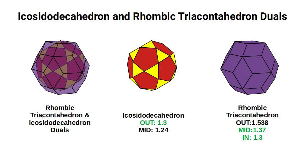
As elements progress from Molybdenum (42) to Technetium (43), there is a shift in dimensionality — from the Truncated Cube and Tetrakis Cuboctahedron to the Truncated Rhombic Dodecahedron and Cuboctahedron compound. When the Octahedron grows in size, this equilibrium changes until a dramatic transformation occurs: the Truncated Cube shifts to an Icosidodecahedron, accompanied by the emergence of the Rhombic Dodecahedron (the 4D hypercube template) in the atomic nucleus. This is the geometric expression of Technetium's instability — the atom is caught between two stable geometric configurations without a stable resting point of its own.

When synthesised in the laboratory, Technetium exhibits several isotopes. The two most stable have neutron counts of 54 and 55 (half-life ~4,200,000 years); the third most stable has 56 neutrons (half-life ~211,000 years). Geometrically, 55 is a Cuboctahedral number: a Cuboctahedron nesting 13 spheres can be surrounded by 42 more to form the next Cuboctahedral shell.

Manganese (25), which appears in the same periodic table group as Technetium (43) in the 1st D-orbital set, also has a nucleon count of 55 (25 protons + 30 neutrons). The Icosidodecahedron has 30 corners; the protons produce a Cuboctahedron of 13 with an additional 12 forming the larger Cuboctahedral shell. This configuration allows Manganese to be stable. The geometry of the 1st D-orbital set is covered in detail in D-orbital Geometry Part 1.

Technetium has 43 protons and can only sustain itself for a limited time before either a neutron transforms into a proton or vice versa. With 54 neutrons, one proton becomes a neutron, producing Molybdenum (42) with 55 neutrons. With 56 neutrons, a neutron becomes a proton, forming Ruthenium (44) with 55 nucleons. With 55 neutrons, one neutron transforms into a proton, again forming an isotope of Ruthenium (44) with 54 neutrons. In every case, the decay moves the atom toward one of the two geometrically stable configurations on either side.

The radioactive nature of Technetium (43) also carries a broader implication: it affects the formation of the F-orbital elements in the same shell. Promethium (61) is the only other element that is naturally radioactive among the stable elements, and it is significant that no D-orbital element in the 2nd set is stable with 61 neutrons. The Icosidodecahedron can be formed by truncating the Dodecahedron or Icosahedron — in the same way the Cuboctahedron is formed by truncating the Octahedron or Cube.

Zirconium (40) and Cadmium (48) sit just before and after the anomaly region and both exhibit exactly the same atomic radius. As elements progress from 40 to 44, the radius falls to 1.3Å; from 45 to 47 it rapidly grows until Silver (47) at 1.6Å. The elements collapse and then rebuild as the set progresses toward completion. This behaviour is not explained by the traditional orbital model, and no existing theory can account for the radioactivity of element 43. More information about these elements can be found in the theory of Harmonic Chemistry, which examines the periodic table from the perspective of music theory.

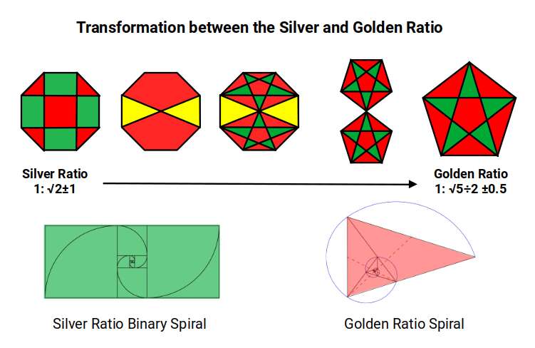
Transition from the Silver to the Golden Ratio

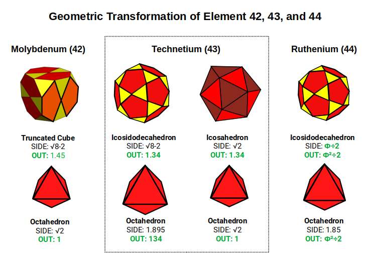
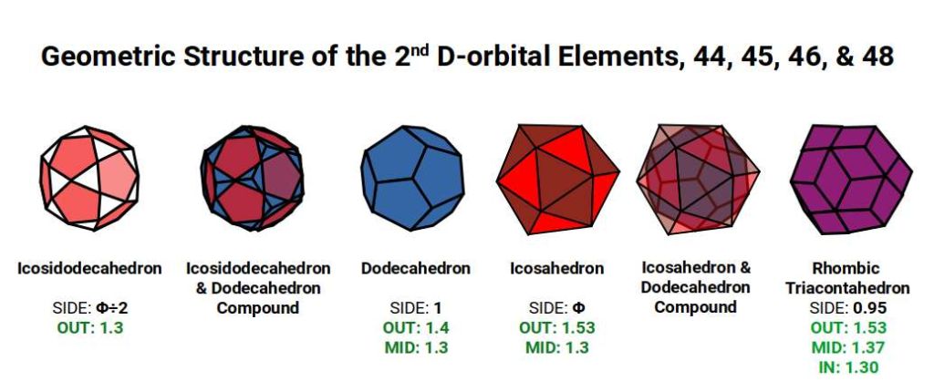
The instability of Technetium (43) is fundamentally a transition between two geometric regimes. The first half of the 2nd D-orbital set — Niobium (41) and Molybdenum (42) — is governed by the Silver Ratio (√2 ± 1), encoded in the octagonal faces of the Truncated Cube. The second half, beginning with Ruthenium (44), transitions to the Golden Ratio (Φ), encoded in the pentagonal symmetry of the Icosidodecahedron. Technetium (43) sits precisely at the midpoint of this transition, unable to resolve geometrically into either ratio.

After Technetium (43), the atomic radius shrinks to 1.3Å for Ruthenium (44) — the smallest radius found in any D-orbital element. Only Osmium (76, in the 3rd D-orbital set) shares this radius, appearing in the same position in its own set.

The geometric transformation from Molybdenum (42) to Ruthenium (44) begins with a Truncated Cube, inside which an Octahedron with a side of √2 is nested. The Octahedron grows in size, pushing through each face of the Truncated Cube and transforming it into an Icosidodecahedron — producing the unstable Technetium (43). An Icosahedron with a side of √2 produces the same sized out-sphere as an Icosidodecahedron with a side of √8 − 2 (which is the Silver Ratio × 2). The Icosahedron can then collapse through the Jitterbug to produce an Octahedron of the same size as that nested in Molybdenum's Truncated Cube — a geometric description of how Technetium decays back into Molybdenum.

The value √8 − 2 = 0.828 is very close to Φ ÷ 2 = 0.809. An Icosidodecahedron with a side of Φ ÷ 2 exhibits an out-sphere of Φ² ÷ 2 = 1.34Å, matching Ruthenium (44). This reduces the nested Octahedron to a side of Φ² × √0.5.

The Golden Ratio is inherent in the pentagon (side 1, diagonal Φ); the Silver Ratio is inherent in the octagon. As elements progress from 42 to 44, the geometry transitions from Silver to Golden Ratio. Element 43, sitting at the exact midpoint of this transition, must either collapse back into the Silver Ratio (Molybdenum) or forward into the Golden Ratio (Ruthenium) — it cannot sustain a stable configuration of its own.

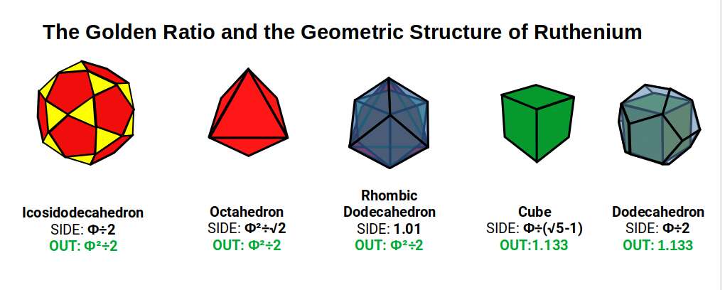
The Icosidodecahedron has 30 corners. Subtracting 30 from Technetium's electron count (43) leaves 13. For Ruthenium (44), the same subtraction leaves 14 — the number of corners in a Rhombic Dodecahedron. This creates a nested pair of the two polyhedra, with the Rhombic Dodecahedron (blueprint for 4D hypercubic space) nested inside the Icosidodecahedron. At this scale, the Cube exhibits a side of Φ ÷ (√5 − 1), with an out-sphere of 1.133Å, nested inside a Dodecahedron with a side of Φ ÷ 2 — beginning the template for the 5D hypercube.

With 5 possible orientations of the Cube within the Dodecahedron (2 orientations, 90° apart, × 5 = 10), and each Cube being a Rhombic Dodecahedron with its octahedral component orientated by the Icosidodecahedron, the 5D cube structure (10 Tesseract cells) maps directly to the geometry of Ruthenium.

This also explains the decay of Technetium (43) into Ruthenium (44): the Icosidodecahedron encodes the Golden Ratio throughout its structure, so it will naturally reduce in size to bring its side length into a Φ:Φ² ratio as the orbitals pass the midway point of the 2nd D-orbital set.

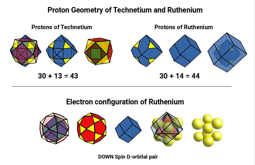
The proton geometry of Technetium (43) consists of a Truncated Rhombic Dodecahedron and Cuboctahedron (30 + 13 corners). For Ruthenium (44), with one extra proton, this shifts to 30 + 14 — two Rhombic Dodecahedra, one truncated to produce 30 corners, nested inside each other to form a 5D hypercube, analogously to how two nested cubes produce a 4D hypercube.

Ruthenium (44) has 7 D-orbital electrons: 5 UP spin completing a full set, and 2 DOWN spin completing two cubic orbitals, reconstructing the 5D hypercube structure (30 + 14 corners). This is why Ruthenium becomes stable: the 5D hypercubic formation begins to complete.

Rhodium (45), Palladium (46), and the Completion of the 5D Template

With the Silver-to-Golden-Ratio transition resolved at Ruthenium (44), the remaining elements of the 2nd D-orbital set build methodically toward the completion of the 5D Hypercubic template. Each step adds both electrons and geometric structure.

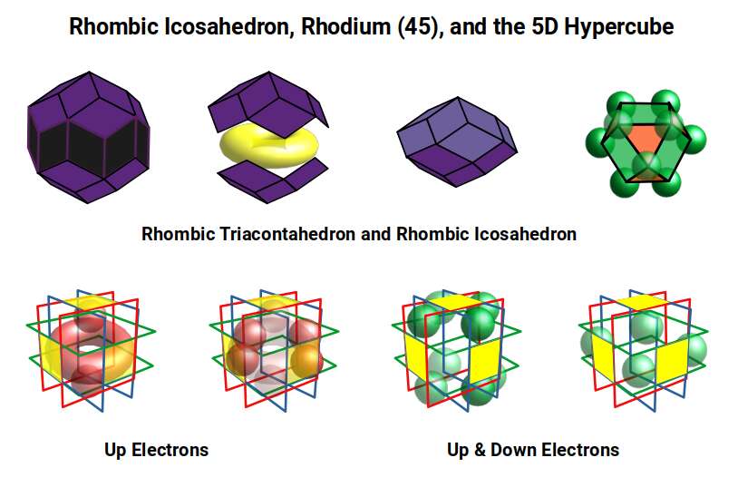
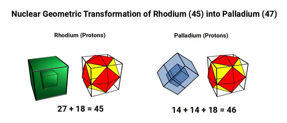
After Ruthenium (44), Rhodium (45) exhibits 8 D-orbital electrons: 5 completing the UP spin set, and 3 DOWN spin electrons completing the Cubic D-orbitals and the template of the 5D Hypercube. The radius increases from ~1.3Å to ~1.35Å.

The dual of the Icosidodecahedron is the Rhombic Triacontahedron — the template for the 6D hypercube, analogously to the Rhombic Dodecahedron for the 4D hypercube. When nested around the Icosidodecahedron (out-sphere 1.3Å), the Rhombic Triacontahedron exhibits a mid-sphere of 1.37Å — closely matching the radius of Rhodium (45).

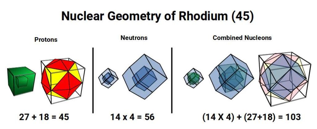
Ruthenium (44) has proton geometry of 30 + 14 corners (Truncated Rhombic Dodecahedron + Rhombic Dodecahedron). For Rhodium (45), the Truncated Rhombic Dodecahedron shifts back to its dual, the Tetrakis Cuboctahedron (18 corners), leaving 27 protons — a cubic number (3³). Rhodium (45) appears in the same periodic table group as Cobalt (27), which also exhibits cubic geometry of 27, covered in D-orbital Geometry Part 1.

A cube of 27 also forms the projection of a 4D hypercube: 1 cube at the centre surrounded by a larger cube formed by the remaining 26 protons. Rhodium has only 1 stable isotope, with 56 neutrons — a multiple of 14 (4 Rhombic Dodecahedra). This produces a nested pair of Rhombic Dodecahedra between the proton geometries, each formed of 3 cubes.

As the electron count passes 44, this shift in geometry is reflected in the electron cloud. The Icosidodecahedron has 30 corners; the Rhombic Triacontahedron has 32. The 45 electrons of Rhodium distribute as 32 + 13, as the Icosidodecahedron shifts toward its dual, with the remaining electron completing the Cuboctahedron — matching the geometry of the completed Cubic D-orbitals.

In geometry, the template for the 5D hypercube is produced by the Rhombic Icosahedron, formed by removing the midsection of the Rhombic Triacontahedron to leave just the top and bottom caps. This midsection corresponds to the torus D-orbitals, which in Rhodium (45) consist only of UP spin electrons. The combination of UP and DOWN spin electrons creates the separation of the two caps, and simultaneously completes the cubic geometry required for the 5D hypercube.

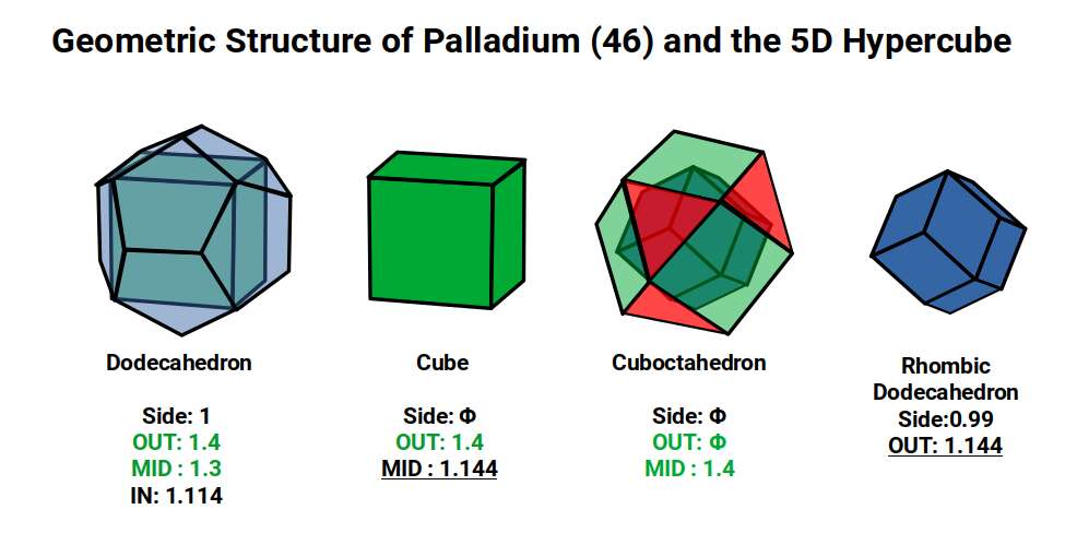
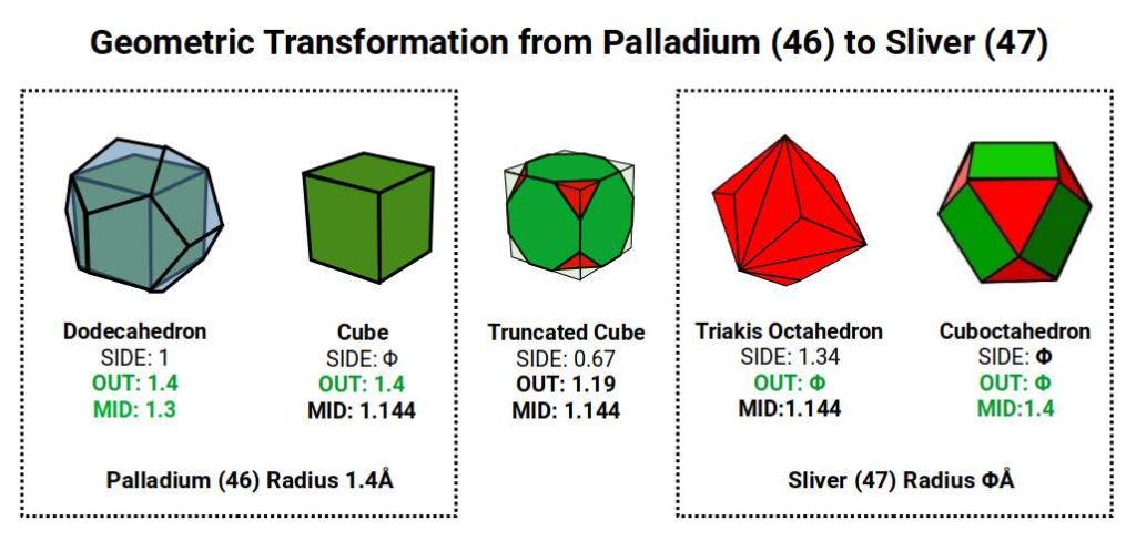
Palladium (46) completes all D-orbital electrons in a single step — the most dramatic Aufbau anomaly in the set. Rather than following the expected configuration of 8 D-orbital electrons and 2 S-orbital electrons, Palladium has 10 D-orbital electrons and no S-orbital electrons whatsoever in its valence shell. It is the only D-orbital element for which this is true. Rather than shrinking, as might be expected when all D-orbitals are filled, its radius is 1.4Å — larger than Rhodium (45) at 1.35Å.

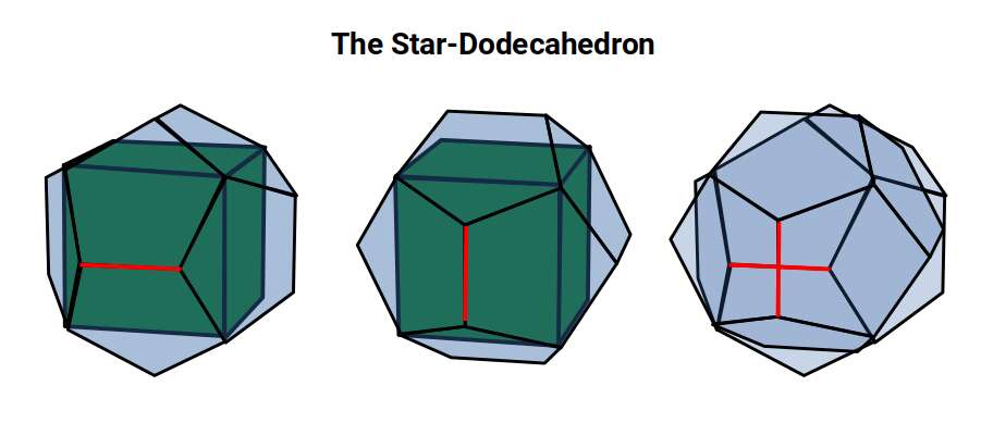
According to Atomic Geometry, the completed D-orbitals are defined by a Dodecahedron with a side of 1, inside which a Cube with a side of Φ is nested. A Cuboctahedron with a side of Φ exhibits a mid-sphere of 1.4Å and an in-sphere of 1.144Å — matching the out-sphere and mid-sphere of the Cube. When the dual Rhombic Dodecahedron is nested within, it also exhibits an out-sphere of 1.144Å. With the Cube nested in 10 orientations (5 in each of the two Star-Dodecahedron orientations), and the same applying to the Rhombic Dodecahedron, the full 5D Hypercubic template is completed at Palladium (46).

Silver (47): The Golden Ratio and Electrical Conductivity

With the 5D template complete at Palladium (46), the set closes with Silver (47) and Cadmium (48) — adding S-orbital electrons back to the outermost shell. Of these, Silver is the more remarkable. Its atomic radius is 1.618Å — the Golden Ratio, Φ — and it is the most electrically conductive element on the periodic table. These two facts are not coincidental.

The Golden Ratio has the unique property that Φ² = Φ + 1 and 1÷Φ = Φ − 1 — in both cases the fractional part remaining the same:

Φ = 1.618… Φ² = 2.618… 1÷Φ = 0.618…

This self-similar property is what makes Φ geometrically exceptional: a structure built at the Golden Ratio can scale indefinitely without losing proportional coherence. In the context of the electron cloud and crystal lattice, this means the geometry propagates through every scale simultaneously.

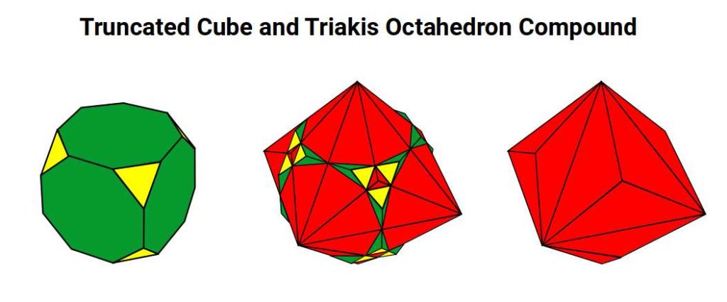
Silver (47) exhibits the geometry of the Tetrakis Octahedron — the dual of the Truncated Cube that governs the 2nd D-orbital set. This dual relationship is significant: the Truncated Cube encodes the Silver Ratio in its octagonal faces, and its dual, the Tetrakis Octahedron, encodes the Golden Ratio in its out-sphere at a side length of Φ — giving Silver both the Silver Ratio geometry of the set's governing form and a Golden Ratio radius.

Silver (47) also exhibits the geometry of the Cuboctahedron through the same relationship observed in the 1st D-orbital set. A cube with a side of Φ both explodes into a Truncated Cube whose dual has an out-sphere of Φ, and collapses through truncation into a Cuboctahedron — both sharing the same geometric proportions. Different 3D projections of the same higher-dimensional form can represent different solids, just as a cube viewed face-on appears as a square and from a corner as a hexagon.

The conductivity of Silver is directly explained by this geometry. Electrical conductivity in metals is described by Brillouin Zones — the reciprocal lattice structure of the crystal. Silver's Tetrakis Octahedron geometry maps onto the Brillouin Zone matrix at multiple scales, producing a fractal correspondence across every level of the structure.

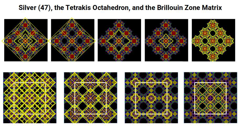
The Brillouin Zone structure encodes both the Silver Ratio and the Golden Ratio. When the electron cloud geometry aligns perfectly with the crystal lattice geometry at multiple scales — as it does for Silver — electrons experience minimal impedance as they propagate through the material. This is the geometric reason that Silver is the most conductive element: not merely a consequence of its electron count or band structure, but a consequence of the fractal resonance between atomic geometry and crystal geometry. The geometric nature of Brillouin Zones is examined in detail in the article on conductive and magnetic properties of elements.

Silver (47) unusually exhibits 2 stable isotopes for an odd-proton element: one with 60 neutrons and one with 62. In the 1st D-orbital set, Copper (29) — which appears in the same periodic table group — also exhibits 2 stable isotopes (34 and 36 neutrons). The parallel is not coincidental: both elements sit at the equivalent position in their respective D-orbital sets, and both have radius values driven by the same class of Golden Ratio geometry.

Overview of the 2nd D-Orbital Set

The 2nd D-orbital set, considered as a whole, traces a complete geometric journey from 4D to 5D space and back again.

The 1st D-orbitals are represented by a Cube of side 1 exploded to form a Rhombic Cuboctahedron of the same side. A Cube of side √2 nests within, with corners at the centre of each triangular face. This contains a Cuboctahedron of side 1, which transforms through the Jitterbug into the Rhombic Cuboctahedron (and passes through the Snub Cube), producing the two main radii of 1.35Å and 1.4Å.

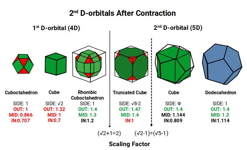
The 2nd D-orbitals begin with a Truncated Cube that can be nested around the 1st D-orbital Rhombic Cuboctahedron when its side length is 1. This entire structure can be placed inside a Cube of side √2 + 1 (the Silver Ratio). The Cube can then be orientated in 5 positions within a Dodecahedron whose side is the Silver Ratio ÷ Φ. However, this model produces out-spheres much larger than those observed:

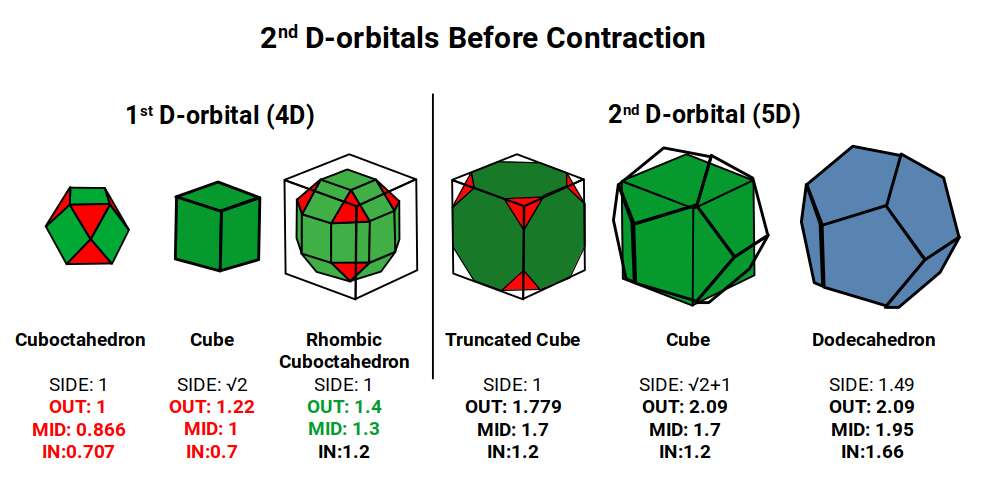
With Niobium (41) and Molybdenum (42), the Truncated Cube forms from a Cube of side 2 rather than 2.414 (= √2 + 1) — reduced by a factor of (√2 + 1) ÷ 2. This gives the Truncated Cube an out-sphere of 1.47Å and a mid-sphere of 1.4Å (the out-sphere of the Rhombic Cuboctahedron of the 1st D-orbital set). Once completed, the Truncated Cube transforms toward its dual, the Tetrakis Octahedron — but as each octagonal face extrudes its midpoint, the Icosidodecahedron forms instead, collapsing the structure at Technetium (43) into the Golden Ratio. After this, the Cube and Dodecahedron build the 5D Hypercubic template, completing at Palladium (46). The Cube's side contracts from 2 to Φ — a reduction by a factor of √5 − 1 — producing an out-sphere closely matching that of the 1st D-orbital Rhombic Cuboctahedron.

The final D-orbital element, Cadmium (48), has a slightly smaller radius than Silver (47) at ~1.55Å. Geometrically, this is produced when the Cuboctahedron with a side of Φ collapses through the Jitterbug into an Icosahedron, yielding an out-sphere of 1.53Å — also the out-sphere of the Rhombic Triacontahedron that defined Ruthenium (44) and Rhodium (45). This is also the same as the out-sphere of the Rhombic Triacontahedron that defined the radii of Ruthenium (44) and Rhodium (45), completing a geometric cycle.

When the structure of elements 44 through 48 is considered together, the Icosidodecahedron with a side of Φ ÷ 2 (out-sphere 1.3Å) and the Rhombic Triacontahedron — formed by the Dodecahedron (side 1) and Icosahedron (side Φ) compound, with a mid-sphere of 1.37Å — define all radii from element 44 to 48, except Silver (47), which has a radius of exactly Φ.

The Rhombic Triacontahedron has 32 corners — the same as the 5D hypercube. The Dodecahedron inside orientates the Cube in 5D hypercubic space in a ratio of 1:Φ. The Icosahedron has a mid-section that rotates independently of the top and bottom caps, producing the torus geometry.

Additionally, the 3rd P-orbitals express a radius of 1.154Å. When these expand through the same Jitterbug-based process used for the 2nd P-orbitals (Cuboctahedron → Snub Cube → Rhombic Cuboctahedron), they produce orbital radii of 1.55Å and 1.61Å, matching the final D-orbital elements in the 2nd set. The mid-spheres of the Snub Cube and Rhombic Cuboctahedron at this scale express 1.3Å and 1.43Å. Note that the radii of Technetium (43) and Rhodium (45) at 1.35Å fall outside this set — confirming their anomalous geometric nature.

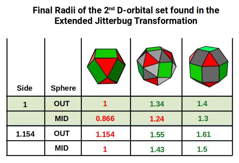
Each set of polyhedra is scaled at a ratio of 1:1.154 — the difference between the mid-sphere and in-sphere of a Rhombic Dodecahedron. The Rhombic Cuboctahedron expresses the qualities of a 4D hypercube; together, the nested pair is indicative of a 5D hypercube. The radii 1.4Å and 1.61Å match Palladium (46) and Silver (47). The larger Rhombic Cuboctahedron then collapses to a Snub Cube with a radius of 1.55Å, matching Cadmium (48). Both the Snub Cube and Rhombic Cuboctahedron have 24 corners, so a nested pair totals 48 corners — the electron count of Cadmium, the final element in this set.

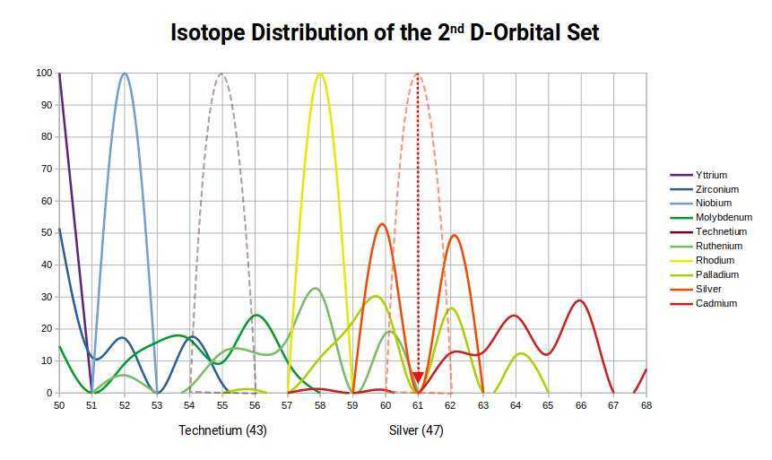
Isotope Patterns and the Number 61

A further regularity across the 2nd D-orbital set merits attention. Compared to the 1st D-orbital set, the 2nd exhibits a larger number of stable isotopes for all elements with an even proton count. Elements with an odd proton count generally exhibit only a single stable isotope. Yttrium (39) is stable only with 50 neutrons; Niobium (41) only with 52. Technetium (43) has no stable isotopes. Rhodium (45) is stable only with 58 neutrons.

There is a significant gap between these neutron counts: the first two odd-proton elements have 50 and 52 neutrons, jumping to 58 for element 45. At the centre of this gap is 55 — the Cuboctahedral number.

No element in the 2nd D-orbital set is stable with 61 neutrons. The same avoidance occurs in the 1st D-orbital set, where the jump in neutron counts similarly skips 61. This is not coincidence: 61 is the first two significant digits of the Golden Ratio (1.618), and the Golden Ratio has the unique property that Φ² = Φ + 1 and 1÷Φ = Φ − 1 — in both cases the fractional part remaining the same. A nucleon count involving 61 cannot be resolved into either a stable Cuboctahedral (55) or Rhombic Dodecahedral (14, 28, 42, 56) configuration. The radioactive nature of Technetium (43) also connects here: Promethium (61) is the only other naturally radioactive element among the stable elements, and its proton count is the same number that the D-orbital isotope distributions avoid.

Conclusion

The 2nd D-orbital set is the most anomalous row in the periodic table by the standards of conventional quantum theory. More elements break the Aufbau Principle than follow it; one element has no stable isotopes at all; and the most electrically conductive element on the periodic table sits in this set with a radius that is precisely the Golden Ratio. Standard quantum mechanics describes these facts but does not explain them — no existing theory predicts them from first principles.

Atomic Geometry explains all three from a single cause: the 2nd D-orbital set is governed by the Truncated Cube, which orientates two Rhombic Cuboctahedra through the Silver Ratio and produces the geometric template for 5D hypercubic space. This dimensional step-up from 4D (the 1st D-orbital set, governed by the Rhombic Cuboctahedron) to 5D is directly encoded in the electron cloud.

The Aufbau anomalies of Niobium (41) and Molybdenum (42) are not exceptions to a rule — they are geometric requirements: the Truncated Cube demands a specific lobe count above and below the torus ring, and the electron configuration conforms to that geometry regardless of what the energy-filling sequence predicts. The instability of Technetium (43) is not a nuclear accident — it is a consequence of sitting at the exact midpoint of the 5D shadow projection, where two Tesseract cells share a middle cube without a stable geometric resolution. The element must decay into either the Silver Ratio geometry of Molybdenum or the Golden Ratio geometry of Ruthenium, because those are the two stable configurations on either side of the transition. And Silver (47), with its radius of exactly Φ and its Tetrakis Octahedron geometry in fractal resonance with the Brillouin Zone lattice, is the most conductive element because its atomic geometry and crystal geometry are aligned at every scale simultaneously — a condition that the standard model of the atom, with its purely electromagnetic account of conductivity, cannot approach.

The broader implication is this: the electron cloud is a multidimensional construct whose radius and configuration are determined by geometry. Electromagnetic forces shape the atom, but they do so within a geometric framework that operates in 4D, 5D, and higher-dimensional space. Until that framework is incorporated into the model, the anomalies of the 2nd D-orbital set — and of the periodic table more broadly — will remain unexplained.

The 3rd D-orbital set (elements 71–80) takes this one step further, building on the 5D template established here to construct the 6D hypercubic geometry. D-orbital Geometry Part 3 examines this transition, the geometry of the Rhombic Triacontahedron as a 6D template, and the exceptional properties of Gold and Mercury that emerge from it.

Related: D-orbital Geometry Part 1 · D-orbital Geometry Part 3 · Atomic Geometry · Brillouin Zones · Harmonic Chemistry

FAQ

Why is Technetium (element 43) radioactive when no other element in the 2nd D-orbital set is?

In Atomic Geometry, Technetium sits at the exact halfway point of the three stable D-orbital sets, where two tesseract cells share a middle cube in the 5D hypercube shadow projection. This geometric instability means the atom cannot sustain its electron configuration and must decay into either Molybdenum (42) or Ruthenium (44), which sit at stable Silver and Golden Ratio geometries on either side.

Why do so many elements in the 2nd D-orbital set break the Aufbau Principle?

The Aufbau anomalies (Niobium, Molybdenum, Palladium and others) arise because the geometry of the Truncated Cube requires a specific number of D-orbital lobes to maintain structural balance. For Niobium (41), one S-orbital electron must transfer to a D-orbital to complete the four-fold cross pattern above and below the torus ring, regardless of what the energy-filling rule predicts.

How can Silver (47) exhibit both the geometry of a Tetrakis Octahedron and a Cuboctahedron?

4D and 5D geometry allow different 3D projections to represent the same form — just as a cube viewed face-on appears as a square, and from a corner as a hexagon. In the 1st D-orbital model, a cube with a side of 1 both explodes into a Rhombic Cuboctahedron and collapses into a Cuboctahedron — both sharing the same side length. For Silver, a cube with a side of Φ similarly transforms into a Truncated Cube whose dual, the Tetrakis Octahedron, produces an out-sphere of Φ, exactly matching the Cuboctahedron of the same side length.

If the Rhombic Triacontahedron is the template for the 6D hypercube, why are the 2nd D-orbitals described as 5D rather than 6D?

Creating a Rhombic Triacontahedron produces only one set of facets of the 6D cube, not the whole structure. The Triacontahedron has 32 corners — the same as a 5D cube — and contains a Dodecahedron that nests 5 Cubes. A full 6D hypercube requires 64 corners, found only in a nested pair of Rhombic Triacontahedra at the correct geometric ratio. The 3rd D-orbital set explores this in more detail.