D-orbital Geometry - Part 1

Introduction

D-orbitals are the third type of electrons to appear in the atom. This article explores the geometric nature of the first set of D-orbital elements (atomic numbers 21–30), and uncovers the geometric reasons for the electromagnetic properties of Iron, Cobalt, Copper, and their neighbours. It is part of a series covering S-orbital geometry, P-orbital geometry, and the broader theory of Atomic Geometry.

This article proposes a single, testable thesis: the 1st D-orbital set — the ten transition metals from Scandium (21) to Zinc (30) — maps geometrically onto two nested polyhedra, the Cuboctahedron and the Rhombic Cuboctahedron. That mapping is not incidental. It directly explains three phenomena that standard quantum theory struggles to account for: why Chromium (24) and Copper (29) violate the Aufbau filling sequence, why Iron (26), Cobalt (27) and Nickel (28) are the only elements ferromagnetic at room temperature, and why the atomic radii of these ten elements cluster tightly around just two values — 1.35Å and 1.4Å — regardless of how large their nuclei grow.

The standard model attributes these anomalies to probabilistic electron shielding and unpaired spin counts. Neither explanation is mathematically complete. What the geometric model offers, for the first time, is a single coherent structure — the Extended Jitterbug, a five-solid transformation sequence — that predicts the radii, explains the anomalies, and accounts for the electromagnetic properties of the 1st D-orbital set from a single geometric framework. The nucleus is not separate from the electron cloud in this model; the geometry of the protons and neutrons drives the observable chemistry.

The article builds in five stages. First, we establish what D-orbitals are and why their cross-shaped lobes map onto a Cuboctahedron. Second, we introduce the Rhombic Cuboctahedron — the second key solid — and show how the pair of them model the full D-orbital set geometrically. Third, we show how atomic radii across all ten elements are predicted by the Extended Jitterbug. Fourth, we use the nuclear geometry to resolve the two Aufbau anomalies. Fifth, we explain ferromagnetism and conductivity as geometric consequences of how the nucleus is structured at Iron, Cobalt, Nickel and Copper. The Conclusion synthesises what this proves and points forward to Part 2.

What is an orbital?

An atom comprises a nucleus of protons and neutrons, surrounded by a field termed the electron cloud. The number of protons and electrons increases in a 1 to 1 ratio to produce all the different types of atoms on the periodic table. This gives each element its atomic number, starting at hydrogen (1) and ending at Bismuth (83), after which the non-stable radioactive elements appear.

Whilst it is common to represent these shells as concentric circles, each containing a certain number of electrons, in truth there are four different types of sub-orbital arrangements. These are labelled S, P, D, and F, each of which forms a particular geometry. This model is based on the Schrödinger equations developed in the 1920s to account for the problems with the concentric ring interpretation of the Bohr model.

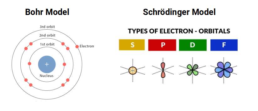
Whilst the Bohr model is still often used to describe the atom, it has been scientifically proven to be incorrect. If the electrons were particles travelling around the nucleus, they would need to be moving faster than the speed of light. Furthermore, the electron's radius has never been established. In more advanced fields of physics, it is more common to treat the electron as a point of charge. Therefore, each orbital lobe represents an area where the electron is likely to be found.

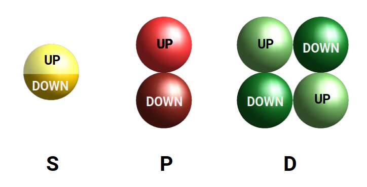
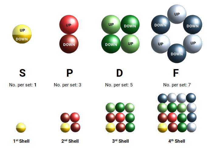
Whilst electrons do not circle the nucleus, they do exhibit a quantum spin value that can be in only one of two states, UP or DOWN. This notion of spin has nothing to do with a rotating particle, and is more accurately described as intrinsic angular momentum. The electron maintains a conservation of angular momentum as if it were rotating, which when aligned with other atoms produces a magnetic field.

When we consider the first three orbital types, a particular geometric pattern emerges. The S-orbital appears as a single sphere made up of two electrons, the P-orbital appears as two spheres either side of the nucleus, and the D-orbitals appear as four. At each step, the number of lobes doubles.

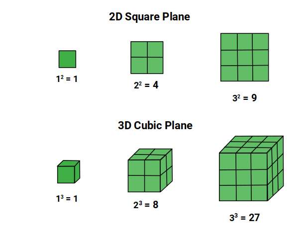
This behaviour exhibits a specific geometric structure that expands through dimension — from the dot (0D) or sphere, to the line (1D), to the square (2D). Our article on 2D orbital geometry explains this in detail, and introduces a 4D geometric interpretation of the electron cloud.

Orbital Configuration

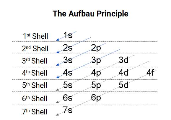
The electron cloud is structured so that for each successive shell, the next set of orbitals is added. The 1st shell holds only two electrons, forming a single S-orbital. The second shell begins by completing an S-orbital, followed by three sets of P-orbitals. The D-orbitals first appear in the 3rd shell, after a set of S-orbitals forms in the 4th.

D-orbitals always come in sets of five. This forms a series of numbers: 1 S-orbital, 3 P-orbitals, 5 D-orbitals. The final F-orbital type comes in sets of seven. In each case, the number of sets expands through an odd number series. As each subsequent shell adds another orbital type, the total number of orbitals in each shell produces a square number series.

The pattern does not continue indefinitely. The 5th shell only forms S, P, and D orbitals, and by the 6th shell only the S-orbitals form as a complete set, along with just three P-orbital elements. This means there are three sets of D-orbitals, appearing in the 3rd, 4th, and 5th shells — accounting for 30 elements, more than any other orbital type.

D-orbital Elements

D-orbitals appear on the periodic table between the S and P-orbitals, in groups 3 to 12. These elements are also called transition metals due to their position. Normally the periodic table lists four blocks of D-orbital elements, however the 4th set is formed of radioactive elements that decay into elements with a lower atomic number. Additionally, element 43 in the middle of the set is also mysteriously radioactive, occurring at the halfway point of the three stable D-orbital sets. Present theory offers no tenable explanation for this occurrence. We will examine this in the 2nd part of this series.

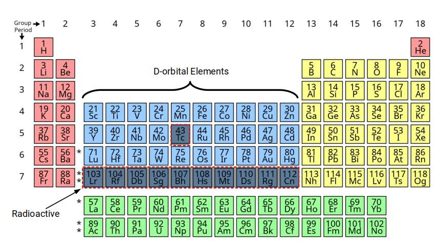
Notice that the standard periodic table places the D-orbital sets in the 4th row. This frequently leads students to believe that the stable D-orbitals appear in shells 4 to 6, rather than 3 to 5, as is actually the case. A more accurate description can be presented by moving the D-orbital set into the correct shell number. Once the radioactive elements are removed from the table, an interesting symmetry begins to emerge.

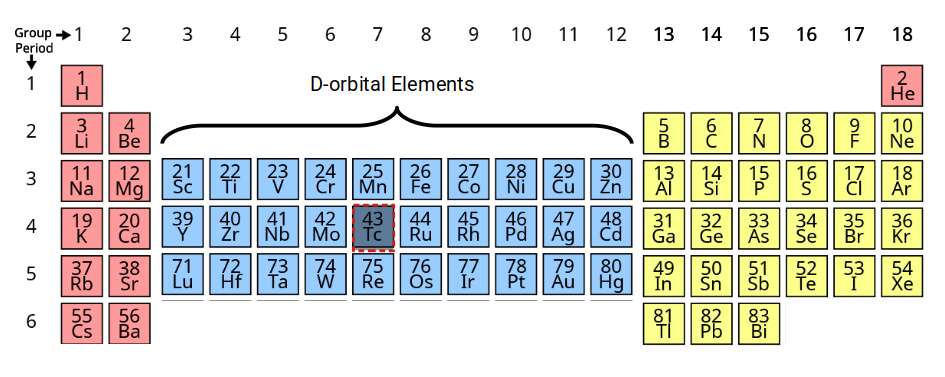
Viewed this way, the D-orbitals are formed inside a shell that already has a complete set of S- and P-orbital elements. The radioactive element Technetium (43) appears at the midpoint: there are exactly 34 elements before it (down to hydrogen) and 34 after it (up to bismuth). This symmetry is not recognised by the traditional model, which uses row-based shell numbering rather than actual electron configuration.

What we will show is that the organisation of these elements has a profound geometric reason, which begins to answer why there are certain anomalies within the structure of the electron cloud. Our theory of Harmonic Chemistry also explores the periodic table from the perspective of music theory.

The Geometric Shape of D-orbitals: From Cross to Cuboctahedron

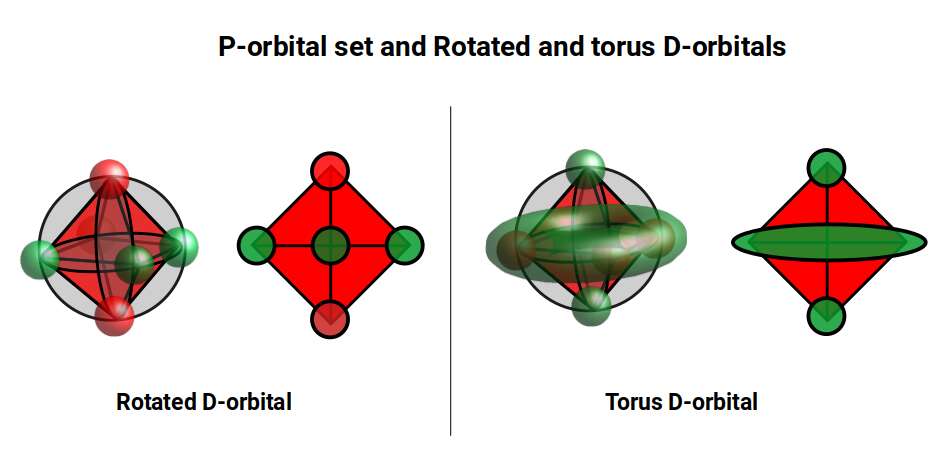
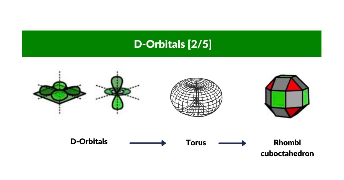
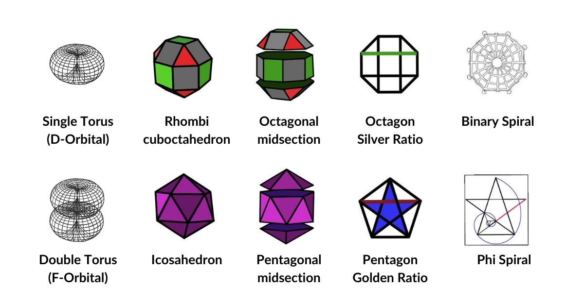
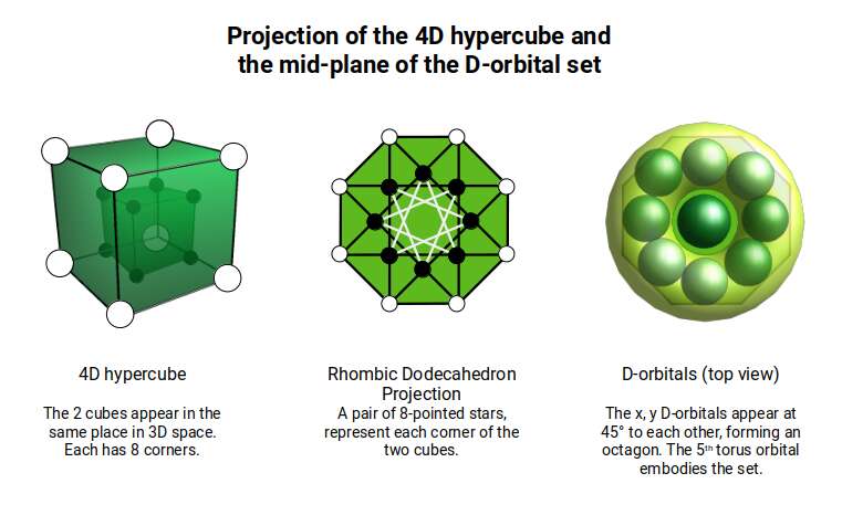
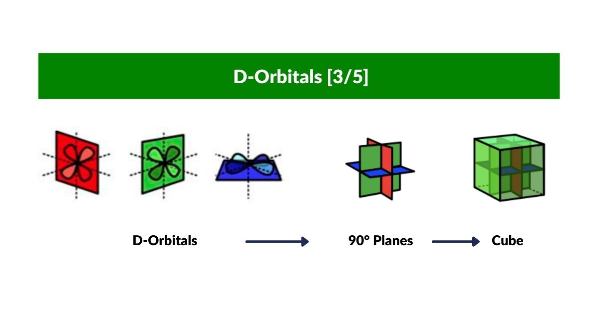
D-orbitals come in a set of five different types. Four are shaped like a cross — two lobes extending in opposite directions from the nucleus — and a fifth appears as a torus shape with a pair of orbital lobes defining the north and south poles. Out of the cross-shaped types, three can be combined to form square planes that divide a cube of space through the x, y, and z axes. The 4th cross-shaped orbital is rotated at 45° on the x, y plane, and falls over the torus orbital ring of the 5th orbital. We can separate these into two sets: three that form the cube, and two that create the torus.

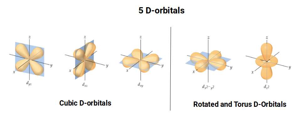
The D-orbitals form after the P-orbitals, which always come in sets of three, each positioned on the x, y, and z axes in the same orientation as the cubic D-orbitals. In the theory of Atomic Geometry, the combined P-orbital set forms the geometry of an Octahedron — a Platonic solid with six corner points. From the perspective of a 4D electron cloud, each P-orbital is assigned the geometry of a torus field wrapping around the edges of the Octahedron. The three cubic D-orbital electrons fall at the midpoints of the Octahedron's sides, dividing it into eight parts.

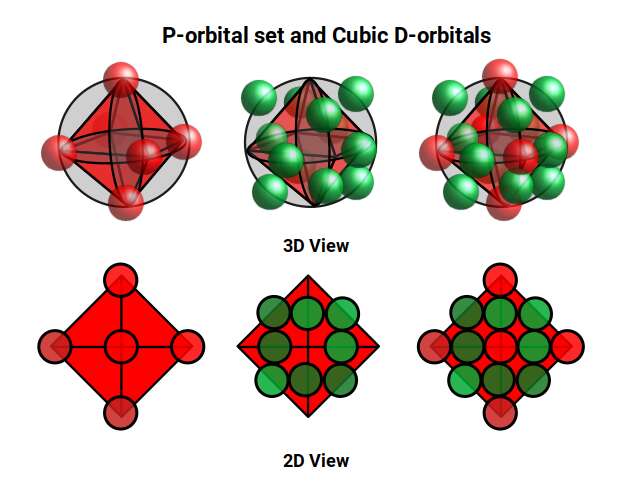
The 4th cross-shaped D-orbital is rotated at 45° on the horizontal plane, appearing superimposed over the two sets of P-orbitals on the x and y-axes. The torus orbital also produces a ring over the same set, with its top and bottom lobe occupying the vertical position where the 3rd P-orbital is found. Therefore, these two D-orbital sets appear in exactly the same orientation as the P-orbitals.

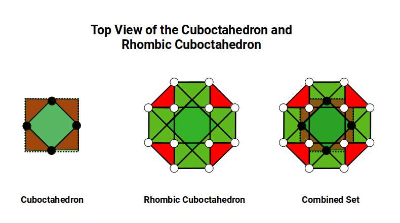
The reason that these D-orbitals appear superimposed over the P-orbital set is not explained by present theoretical models. Yet the result is an ordered geometric configuration that can be mapped to two nested 3D polyhedra: the cubic D-orbitals fall into the space in between the P-orbitals, defining a Cuboctahedron, whilst the rotated and torus orbitals fall in the same place as the P-orbitals, represented by an Octahedron.

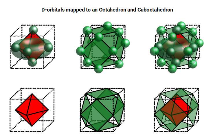
In our examination of P-orbital Geometry, we explained how the Octahedron transforms into a Cuboctahedron through the Jitterbug Transformation. The D-orbital set appears to map both of these combined polyhedra in a single orbital set.

4th Dimensional D-orbital Geometry

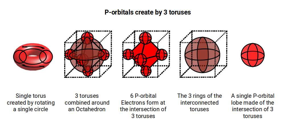
The appearance of the torus-shaped D-orbital is suggestive of the 4D nature of the electron cloud. The torus is a 4D shape generated by a circle (or sphere) that is rotated around a central axis to complete the form. In our examination of P-orbital sets, we attribute the mysterious movement of the electron from one orbital lobe to the other to the unification of two toruses oriented at 90° to each other. By the time the P-orbital set completes, three toruses form around the sides of the Octahedron, and each P-orbital lobe is defined by three intersecting circles forming the internal geometry of a sphere.

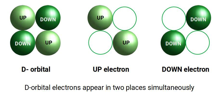
The D-orbitals all form within the toruses of the P-orbital set. Each cross-shaped D-orbital is comprised of two electrons with either an UP or DOWN quantum spin value. When measuring the particle, the act of observation can only determine a single location. If we separate the two lobes, each electron falls into two places simultaneously — indicating that the electron is not a particle as commonly presumed, but is present in two places at the same time.

This concept has nothing to do with quantum superposition, which is derived from the nature of electron spin. The standard model treats orbitals as probabilistic, but does not consider the electron as a purely wave phenomenon. This is partly because current theory disregards the background energy of space, sometimes referred to as the Aether.

Yet the vacuum energy is a scientific fact and is the reason why the speed of light is constant. Once we reintroduce the notion of this energy field, the orbitals begin to take on a more defined nature. Each lobe represents an area of increased energy density generated by the quantum ½-integer spin values of the field. For every 360° rotation in 3D space, the electron must rotate 720°. These are sometimes described as Spinors, however from a geometric perspective, this nature can be accounted for by the rotation of a 4D polytope — as explained in our article on the 4D electron cloud.

The Rhombic Cuboctahedron: The Second Key Solid

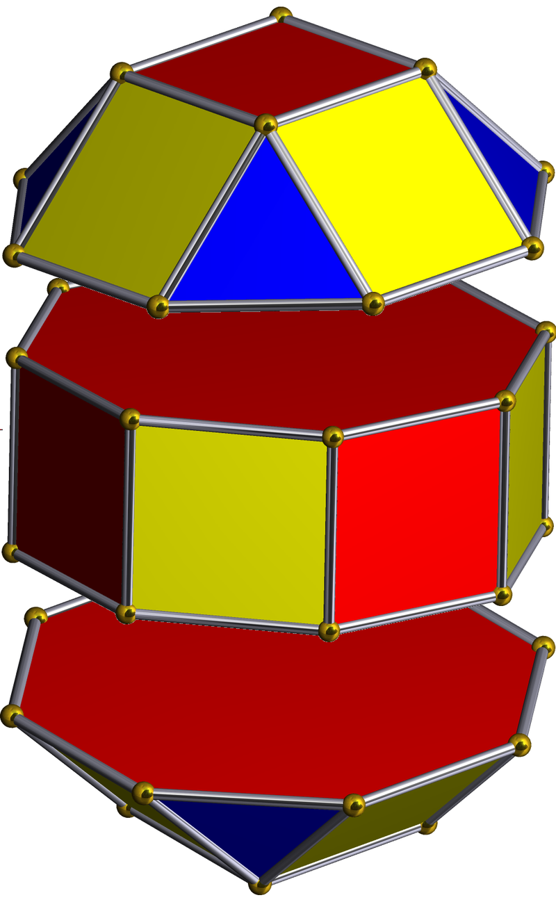
Whilst the cross-shaped D-orbitals map cleanly onto the corners of a Cuboctahedron, the torus-type orbitals require a second solid to complete the picture. That solid is the Rhombic Cuboctahedron — an Archimedean solid composed of the faces of a Cube and Octahedron that have moved away from the centre, leaving 12 additional square spaces. The result is a polyhedron with 24 corners, 8 triangular faces, and 18 square faces.

The unique quality of the Rhombic Cuboctahedron, and the reason it is assigned to the torus D-orbitals, is that it is the only Archimedean Solid with an octagonal midsection. This prism is free to rotate between its two caps in 45° increments — exactly like the orientation of the D-orbitals on the central plane. No other Archimedean solid has this property.

Aside from the Rhombic Cuboctahedron, the only Platonic Solid with a similar rotating quality is the Icosahedron. The former exhibits square faces and forms an octagon (generating the Silver ratio, √2±1), whilst the Icosahedron's pentagonal midsection expresses the Golden ratio, (√5÷2)±½. In Atomic Geometry, the Rhombic Cuboctahedron is assigned to the D-orbital torus, whereas the F-orbitals exhibit a double torus mapped to the Icosahedron.

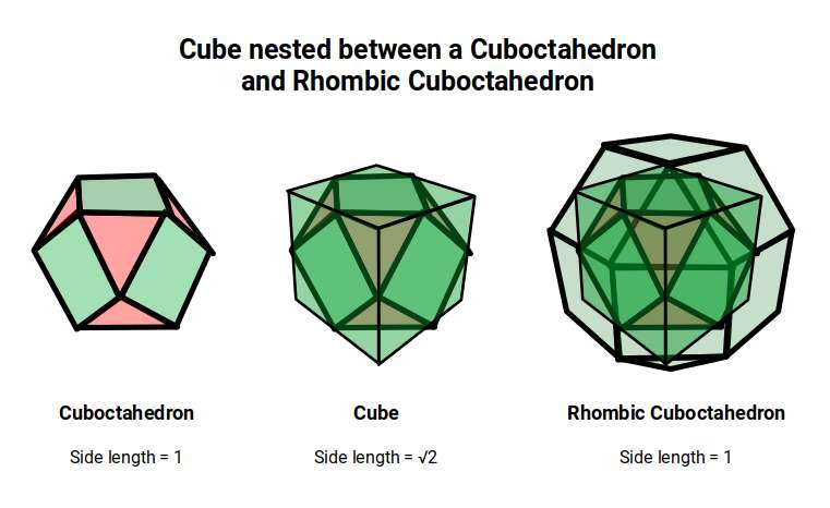
The two key solids — the Cuboctahedron and the Rhombic Cuboctahedron — are geometrically related through a nested structure. A Cube can be nested inside a Rhombic Cuboctahedron so that its corners touch at the centre of each triangular face. If the Rhombic Cuboctahedron has a side length of 1, the Cube will have a side of √2. Additionally, a Cuboctahedron can be formed by truncating the corners of the Cube to a side length of 1. In this way, the complete set of orbitals can be perfectly oriented within this nested set of polyhedra: the Cuboctahedron (inner) models the three cubic D-orbitals, the Cube (√2) forms the connecting structure, and the Rhombic Cuboctahedron (outer) models the torus pair.

4D Geometry and the Silver Ratio

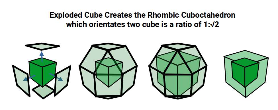
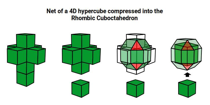
The geometric relationship between these two solids extends into four dimensions. The 4D hypercube can be envisioned as two cubes superimposed over the same space in 3D. In the geometric model of the D-orbitals, two cubes are oriented by the Rhombic Cuboctahedron. As shown previously, this polyhedron can be formed by exploding a cube so that its faces expand away from the centre. If the initial cube has a side length of 1, the second will be √2 larger.

Just as a 3D polyhedron can be created by cutting out a 2D template and folding it, the same applies to 4D solids. The Tesseract (4D Cube) is formed by a similar net to the 3D Cube, except the six square faces are replaced by eight Cubes. A 4D polytope has 3D shaped faces. This template forms a 3-dimensional cross in space that is folded in 4D. Notice how the outermost cube wraps around the others, which corresponds to the concept of two Cubes nested inside each other.

We can compare this net to the model of the Rhombic Cuboctahedron. The cube that wraps around the others is already defined by the √2 Cube nesting with its corners touching the triangular faces of the Rhombic Cuboctahedron. Detaching this leaves a central Cube with six more attached to each face, forming along an x, y, and z axis — similar to the P-orbitals. By contracting each outer cube towards the centre, the shell of the Rhombic Cuboctahedron forms. In this way, we can begin to recognise how the Rhombic Cuboctahedral structure can represent the formation of a 4D hypercube.

The Rhombic Cuboctahedron produces an octagon when viewed from above, exhibiting the Silver Mean (√2±1). Similar to the Golden Mean, the unique quality of this ratio is that its reciprocal value switches the equation to the negative: √2+1 = 2.414…, with a reciprocal of 0.414…, or √2-1. This gives it a particular fractal quality that can collapse into infinity through the Silver Spiral.

If the outer cubes in the Rhombic Cuboctahedral construction remain the same size as they contract, a small cubic space forms at the centre with a side length of √2-1. The structure can be enclosed in a cube with a side length of √2+1. Together with the nested cube (side √2) and original cube (side 1), this produces a perfect expression of the Silver Ratio within the Rhombic Cuboctahedral structure.

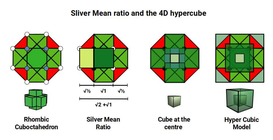
This model of nested solids provides an insight into the geometric nature of the D-orbitals. The three cubic cross-shaped orbitals form at the midpoints of the cube's sides, defining the Cuboctahedron. The remaining two form the torus field of the Rhombic Cuboctahedron, which orients a larger cube (√2) by anchoring its corners upon the triangular faces. The octagonal midsection accommodates the 4th set of cross-shaped D-orbitals, oriented at 45° to the others.

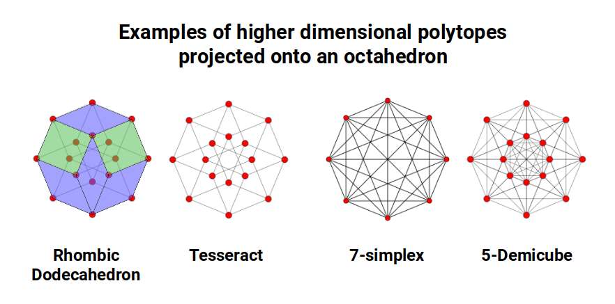
The Octagon is recognised for its capacity to produce a shadow projection of the 4D tesseract, and can be used to define a variety of higher-dimensional polytopes, including the 7th-dimensional Simplex and the 5D Demicube, both based on the Tetrahedron.

4D Hypercube and the Rhombic Dodecahedron

Before continuing, let us consider the nature of higher-dimensional space. A 4D hypercube can be rotated on the familiar x, y, and z axes, but also exhibits a fourth w ('time') axis. When rotated on its w axis, the cube will 'swap' places in 3D space as it rotates.

Another way to visualise a 4D object is to pass it through a 3D space. For example, a Cube passed face-on through a 2D plane will create a square the moment it touches the surface. The square will exist for a certain period of time dependent on the speed of passage, then vanish. We can apply a similar concept to a 4D hypercube passed through a 3D hyperplane.

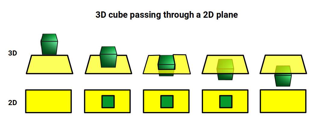
Interestingly, each of these projections can be ascribed to the three types of lattice structures formed by D-orbital element compounds. The face-on projection forms a cubic shell similar to the Face Centred Cubic (FCC) structure, the side-on view forms a Hexagonal Close Packing (HCP) cell, and the w-axis exhibits a cube at its centre, indicative of the Body Centre Cubic (BCC) configuration. We will discuss these in more detail at the end of the article.

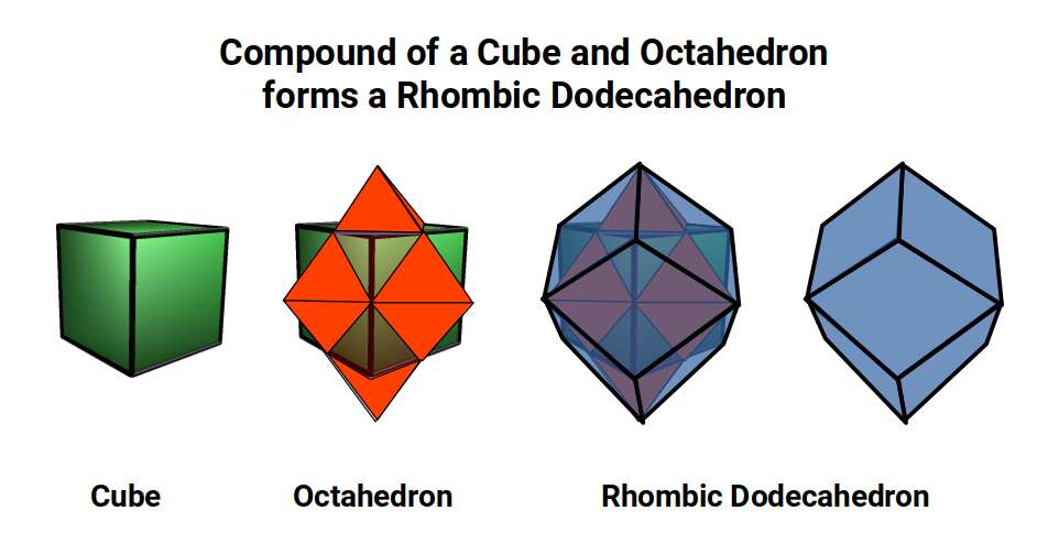
The dimensions of the dark blue frame outlining the tesseract's passage through the 3D plane can be defined by a Rhombic Dodecahedron, formed from the compound of the Cube and Octahedron.

D-orbital and the Hypercube

The Cube is the only Platonic solid that can fill space completely by itself. Similarly, the 4D hypercube tiles 4D space, and its equivalent tiling in 3D is produced by the Rhombic Dodecahedron. 13 Rhombic Dodecahedra can be compiled in 3D space in an Octahedral formation (actually forming a Truncated Octahedron). By adding another six (total 19), the Octahedral shape becomes complete.

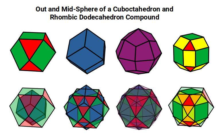
The 4D hypercube (tesseract, or 8-cell) can be envisioned as two cubes occupying the same 3D space. The Rhombic Dodecahedron represents the midpoint in the transition from one Cube to the other. At the centre of the offset cubes, a small square forms which, when projected onto a flat surface, produces an 8-pointed star. This is similar to the small cube that forms at the centre of the Rhombic Cuboctahedral structure explored previously. In fact, the shadow projection of the Rhombic Dodecahedron projected onto a flat surface generates the same image as our nested Rhombic Cuboctahedral image of the D-orbital set.

The conclusion is that both the Rhombic Dodecahedron and the Cuboctahedron are expressions of a 4D hypercube. Whereas the Rhombic Dodecahedron forms the template and can fill 3D space perfectly by itself, the Rhombic Cuboctahedral model exhibits the Silver Ratio, is composed of two cubes, and exhibits the notion of a torus — with its mid-plane rotated at 45°, just like the D-orbital set.

Atomic Radii of the 1st D-orbital Set

With the geometric model established, we can now test it against measured data. The radius of each element is defined by two main theoretical models. The Van der Waals radius treats the atom as a hard spherical shell, offering a much larger radius than experimentally determined values and not accounting for D-orbitals. The only theoretical prediction for D-orbital elements is derived from the Bohr model. However, the predictions for D-orbitals are out by a factor outside the margin for experimental error. The atomic radius is measured in Angstroms (Å), where one unit is equivalent to about 100 picometres. The margin of error for experimentally determined radii is ±5Å, and when we graph both datasets the difference is quite substantial.

In all cases, the Bohr Model consistently predicts a larger radius for D-orbital elements than has been experimentally verified. At best, only Silver (47) — an unusually large atom — falls near the upper boundary. The discrepancy is traditionally attributed to D-block contraction: D-orbitals form in the shell below a completed S-orbital set and can shield the outermost electron as more protons are added. However, investigation into the exact mathematical equations justifying this view reveals them to be largely absent. There is no viable model that explains why so many D-orbital elements appear at roughly the same size.

This becomes even more apparent when we compare the experimentally determined radii across all three D-orbital sets. The 7th element of each set is exactly the same size, despite vastly different nuclei. Cobalt (27) in the 1st D-orbital set has 27 protons and 32 neutrons — a nucleus dramatically different from the corresponding elements in the shells above — yet the radius remains consistently at 1.35Å.

Mapping Radii to the Rhombic Cuboctahedral Model

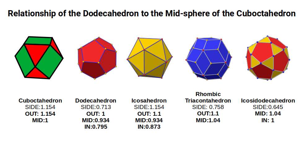
The Rhombic Cuboctahedron model of the D-orbitals nests five different solids: three cubes (sides 1, √2, and √2+1), plus a Cuboctahedron and Rhombic Cuboctahedron, both with side length 1.

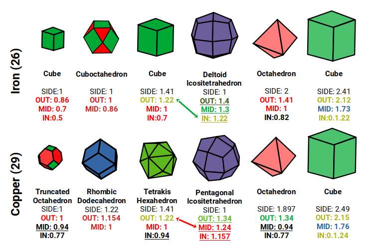
Each Cube exhibits an in-sphere, mid-sphere, and out-sphere. The out-sphere wraps around the Cube's corners, the mid-sphere touches the middle of the sides, and the in-sphere touches the centre of each face. The same concept applies to other polyhedra. Based on a Cube with a side of 1, we can map the dimensions of all spheres created by the Rhombic Cuboctahedral model.

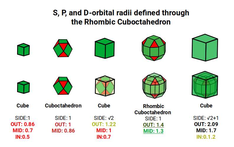
A Cube with a side of 1 produces in, mid, and out-spheres that closely match the radius of many 1st P-orbital elements. The Cuboctahedron defines the space between the largest of the 1st P-orbital set and the smallest of the 2nd. The √2 Cube has an out-sphere of 1.22Å — the radius of Helium (2), the only S-orbital noble gas, and completely non-reactive. Beyond this, the Rhombic Cuboctahedron exhibits a mid-sphere of 1.3Å (the smallest D-orbital element) and an out-sphere of 1.4Å (matching four of the 1st D-orbital radii and the final elements of the 4th P-orbital set). The geometric model provides a much closer match in most cases than the Bohr radius, which shows significant inconsistencies for Helium, the latter half of the 2nd S-orbital set, and all D-orbital elements.

The Extended Jitterbug and the Two D-orbital Radii

The nested model of the Rhombic Cuboctahedron establishes the geometry. The Extended Jitterbug transformation explains how that geometry changes as successive D-orbital elements form — and in doing so, predicts the precise radii at which the changes occur.

In our previous article on P-orbitals, we explored the Jitterbug transformation described by Buckminster Fuller. This process transforms an Octahedron into a Cuboctahedron by opening its sides to create triangular and then square faces. As the distance between corners reaches 1, the Icosahedron forms; as it increases to √2, the square faces of the Cuboctahedron appear. Just like a 4D polytope, this structure can collapse, flipping itself inside out.

Whilst the Jitterbug is relatively well documented through the work of Buckminster Fuller, what is not commonly recognised is that the sequence can be extended to incorporate two more solids — the Snub Cube and Rhombic Cuboctahedron. We call this the 'Extended Jitterbug'.

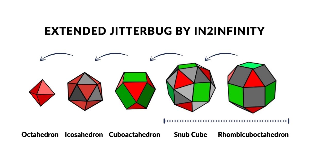
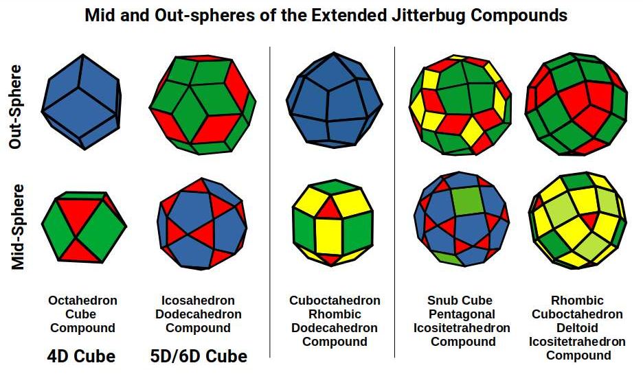
The Extended Jitterbug is formed of five polyhedra, with the Cuboctahedron at its centre and the Rhombic Cuboctahedron as the largest. Both solids assigned to the D-orbital sets can be transformed from one to the other through the Snub Cube. The Cuboctahedron can collapse into the Icosahedron (which, like the Rhombic Cuboctahedron, has a mid-section that can be rotated), and finally into the Octahedron — the smallest solid in the set, representing the P-orbital geometry.

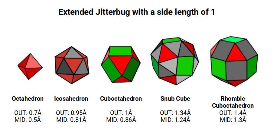
The Extended Jitterbug also produces striking correlations to atomic radii. Based on an Octahedron with a side of 1, the expansion through the Jitterbug produces a Rhombic Cuboctahedron in the same proportion as the exploded model. The out and mid-spheres define the gap between the largest 1st P-orbital elements and the smallest of the 2nd set. The Cuboctahedron collapse to the Octahedron defines the radius of Carbon (6) at 0.7Å and Fluorine (9) at 0.5Å.

This model reveals the second major radius found in the 1st D-orbital set: 1.35Å. Except for Scandium (21) at ~1.6Å, all other 1st D-orbital elements exhibit a radius of either 1.4Å or 1.35Å — corresponding to the out-spheres of the Snub Cube and Rhombic Cuboctahedron in the Extended Jitterbug model. These are not approximate coincidences; they are the direct prediction of the model. The question is why the radius shifts from one to the other at specific elements — and the answer lies in the nuclear geometry, which we examine next.

The Aufbau Anomalies: A Geometric Explanation

The order by which electrons fill the atomic structure is usually described by the Aufbau Principle. D-orbital elements exhibit two significant anomalies in this sequence. Chromium (24) has only one S-orbital electron in its outer shell, with a counterpart mysteriously appearing as an extra D-orbital, completing the torus D-orbital set prematurely. The same anomaly occurs with Copper (29), which again appears with only a single outer S-orbital electron and a full D-orbital configuration. Standard theory attributes these anomalies to electromagnetic shielding effects — but no mathematical model precisely derives when or why these interruptions occur.

When the orbital types are divided into three cubic and two torus types, the anomalies become explicable without any electromagnetic assumption. The first three D-orbitals form the cubic set; the next element adds two D-orbitals to complete the torus set.

As the first three D-orbitals form, the atomic radius reduces to 1.35Å (the out-sphere of the Snub Cube). With the 4th element, Chromium (24), the radius increases to 1.4Å as the Snub Cube expands into the Rhombic Cuboctahedron. The Rhombic Cuboctahedron has 24 corners — the same as the number of protons in Chromium. Its total nucleon count is 52, which is divisible by 13, the number of spheres nested within a Cuboctahedron.

The same anomaly occurs with Copper (29). When we examine the atomic nucleus, we find 29 protons and 36 neutrons, totalling 65. Like Chromium's nucleus, this number is also divisible by 13. Therefore, in the 1st D-orbital set, the two atoms that exhibit Aufbau anomalies both have a nucleonic count divisible by 13 — the number of spheres nested by a Cuboctahedron.

This is a completely new perspective that resolves the Aufbau Anomalies, not through mysterious electromagnetic interactions and 'shielding' as is commonly taught, but through a purely geometric mechanism: when the nucleus contains a nucleon count divisible by 13, the geometry of the Cuboctahedron drives a premature completion of the D-orbital set.

Evidence supporting this comes from the atomic nucleus. All elements between the two anomalous atoms exhibit a neutron count of 30, with one exception: Cobalt (27) with 32. After Nickel (28) with 58 nucleons, the anomalous Copper (29) appears with 65. This large jump in nucleus size is not matched by an increase in radius — the atom remains at 1.35Å. This fact is difficult to accommodate within conventional theory.

Nuclear Geometry of the 1st D-orbital Set

To understand why these anomalies happen at these specific elements, and why ferromagnetism appears at Iron, Cobalt and Nickel rather than at Chromium or Manganese, we need to examine the nuclear geometry element by element. In the theory of Atomic Geometry, the nucleus plays an important role in explaining the different qualities expressed by a particular element. Geo-nuclear Physics focuses particularly on the number of neutrons and protons that constitute a stable atom.

Scandium (21) exhibits the largest radius of any 1st D-orbital element at 1.6Å, a value close to the Golden Ratio (Φ ≈ 1.618). This larger size is due to the D-orbitals only just beginning to form, with the radius reducing from the even larger S-orbital elements Potassium (19) and Calcium (20) at 2.2Å and 1.8Å respectively.

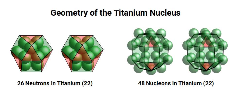
After this, the radius drops to 1.4Å for Titanium (22), which is stable with 26 neutrons. A Cuboctahedron can nest 13 spheres perfectly in space, with 12 surrounding one at the centre. As 26 = 2×13, the neutron count equals the spheres nested by two Cuboctahedra. The 26 neutrons bring the total nucleon count to 48, which is the number of corners found in two Rhombic Cuboctahedra. Thus the nucleus of Titanium (22) is a perfect match for the geometric model.

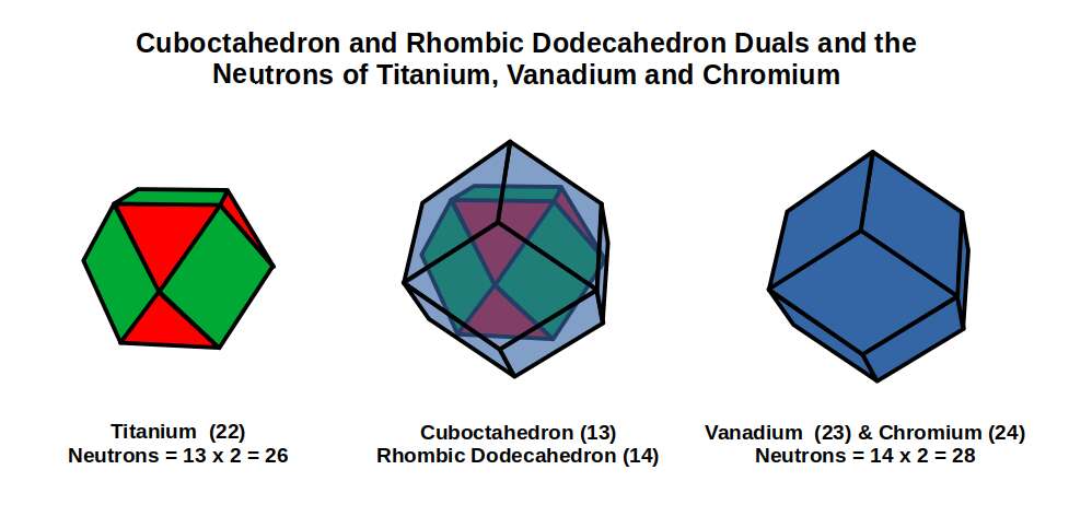
The subsequent element, Vanadium (23), exhibits a slightly smaller radius of 1.35Å. For the next element, Chromium (24), the radius increases back to 1.4Å. Both have 28 neutrons, divisible by 14 — the number of corners of a Rhombic Dodecahedron. Geometrically, the neutrons of Titanium (22) exhibit a Cuboctahedral structure, which morphs into its dual for Vanadium (23) and Chromium (24).

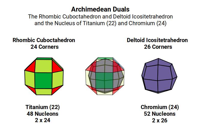
When we count the total nucleons for Vanadium (23) and Chromium (24), the totals are 51 and 52 respectively. As 52 = 4×13, the Chromium nucleus geometrically forms four Cuboctahedra — which translates to the corners of two Deltoid Icositetrahedra (the dual of the Rhombic Cuboctahedron). From Titanium (22) to Chromium (24), the nuclear geometry transforms into its dual.

The reason for the slight dip in radius for Vanadium (23) can be attributed to the fact that 23 is an odd number, leaving not quite enough protons to complete the Rhombic Cuboctahedron, causing the structure to collapse into the Snub Cube. Titanium (22) has 48 nucleons (12×4) — the corners of four Cuboctahedra. Chromium (24) has 52 nucleons (13×4) — filling in the missing central sphere of each. Vanadium (23), appearing between them, can only fill three of the central spaces, leaving the fourth empty and causing the geometric collapse that reduces its radius to 1.35Å.

Chromium (24) exhibits 24 protons and 28 neutrons — a perfect ratio to form the 24 corners of a Rhombic Cuboctahedron and two Rhombic Dodecahedra. At this point, the D-orbital set suddenly completes, creating the 1st Aufbau Anomaly. The geometry drives the anomaly directly: 52 = 4×13 is the condition, and the D-orbital set must complete when the nucleus reaches it.

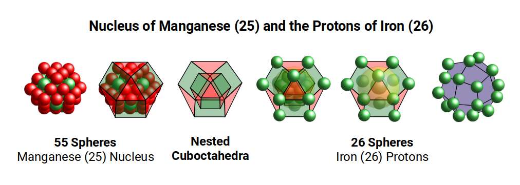
After this, Manganese (25) forms, marking the halfway point in the D-orbital set with 55 nucleons. Just as a Cube can be formed of 8 (2³) or 27 (3³) units, a Cuboctahedron expands from 13 to 55 units (the Cuboctahedral numbers), which is a recognised magic number in chemistry and nuclear physics.

Examining these first five elements, we can see the nucleus transforming through a geometric process. Beginning with Scandium (21) with 24 neutrons (corners of a Rhombic Cuboctahedron), subsequent elements transform through the Cuboctahedron, Rhombic Dodecahedron, and their duals, until a large Cuboctahedral structure with the magic number 55 forms in Manganese. The neutron count then increases to 30, ascribed to the 30 corners of the Icosidodecahedron, which is important in the transition from a 4D to 5D hypercube.

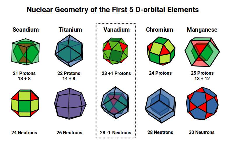
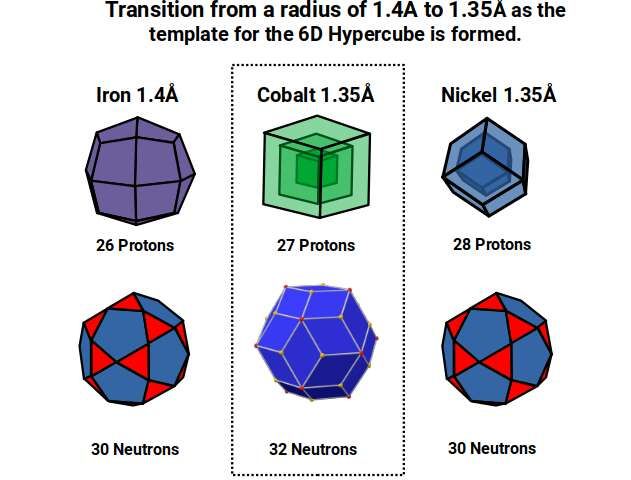
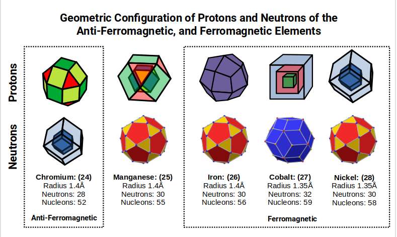
After Manganese (25), Iron has the same number of neutrons but 26 protons (2×13, or the corners of a Deltoid Icositetrahedron — the same geometry as the neutrons in Titanium). This is the final D-orbital element in this sub-set, with a radius of 1.4Å.

After Iron (26), the radius collapses to 1.35Å for Cobalt (27). The 27 protons form a Cube with a side length of 3, just like the neutrons of Vanadium (23). The neutron count for Cobalt (27) increases from 30 to 32, ascribed to the corners of the dual of the Icosidodecahedron, the Rhombic Triacontahedron — which forms the template for the 6D hypercube in the same way the Rhombic Dodecahedron forms the template for the Tesseract.

Nickel (28) has 28 protons (the same as the neutron count of Vanadium and Chromium), depicted as two nested Rhombic Dodecahedra. Once the proton count passes 27 to form a hypercubic structure, the protons divide into two nested solids, and the neutron count suddenly drops back to 30. There is presently no explanation for why Nickel should exhibit two fewer neutrons than Cobalt yet maintain exactly the same radius. Geometrically, this represents the collapse of the Rhombic Icosidodecahedron (6D hypercube template) back into its dual, the Icosidodecahedron, as we pass the number 27.

The neutron count in the final two elements, Copper and Zinc, increases dramatically. The Pentagonal Icositetrahedron — the dual of the Snub Cube — has 38 corners. Copper comes in two forms (isotopes) with 34 or 36 neutrons (roughly 70%/30% ratio), giving an average of approximately 35 neutrons. Subtracting 38 from the nucleon counts (63 and 65) leaves remainders of 25 and 27 — reflecting the proton counts of Manganese (25), Cobalt (27).

Zinc (30) has 30 protons, the same number as the neutron count of Manganese, Iron, and Nickel — represented by the Icosidodecahedron. Zinc exhibits three main isotopes with neutron counts of 34, 36, and 38. Subtracting 38 from each produces remainders of 26, 28, and 30 — echoing the proton counts of Iron, Nickel, and Zinc itself.

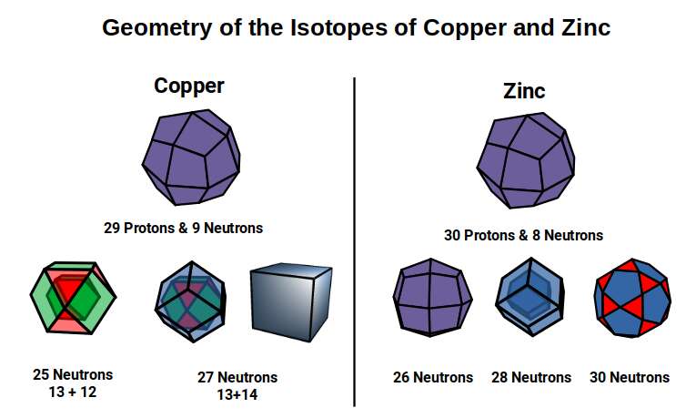
Notice that the last Zinc isotope produces a perfect geometric division between 30 protons (Icosidodecahedron) and 38 neutrons (Pentagonal Icositetrahedron). After this, the D-orbital elements complete and the next P-orbital set begins. When comparing the first and second halves of this D-orbital set, the neutrons in the first half tend to transform into the proton count in the second half as the nuclear geometry evolves.

The Collapse of the Rhombic Cuboctahedron into the Snub Cube

After Iron (26), all remaining 1st D-orbital elements express a radius of 1.35Å. This shift is represented geometrically as the collapse of the Rhombic Cuboctahedron into the Snub Cube, as part of the Extended Jitterbug transformation towards the Cuboctahedron.

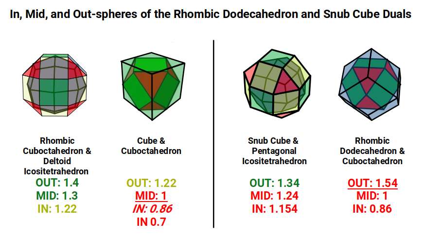
When the Rhombic Cuboctahedron creates a nested set with its dual, the Deltoid Icositetrahedron, in, mid, and out-spheres are produced. The same applies to the Snub Cube and its dual, the Pentagonal Icositetrahedron. Examining the radius of each set reveals strong correlations to many atomic radii.

Set to a relative side length of 1, the out-spheres of both sets define the two main atomic radii found in the 1st D-orbital set. The in-sphere of the Rhombic Cuboctahedral pair exhibits a radius of 1.22Å (approximating Helium, the 1st atomic shell). When the Rhombic Cuboctahedron collapses into the Snub Cube, the out-sphere reduces to 1.35Å (the second main D-orbital radius). The mid-sphere drops from 1.3Å to 1.24Å, and the in-sphere to 1.154Å — an exact match for the 3rd P-orbital set that forms directly after the 1st D-orbital set (Gallium, 31 at 1.3Å; Germanium, 32 at 1.25Å; Arsenic, Selenium, and Bromine at 1.154Å).

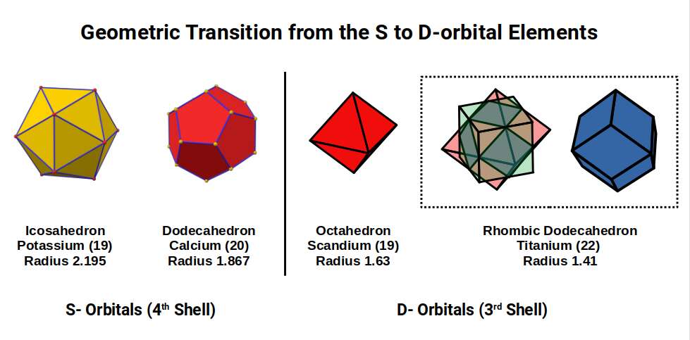
The transition of the P-orbitals from 1Å (3rd shell) to 1.154Å (4th shell) offers a geometric explanation for the large jump in S-orbital radii: Potassium (19) at 2.2Å, and Calcium (20) at 1.8Å. An Octahedron can nest a Cuboctahedron perfectly in its mid-sphere. If the Cuboctahedron has a side of 1.154, the enclosing Octahedron has a side of 2.3Å, producing an out-sphere of ~1.63Å — roughly the radius of Scandium (21). This Octahedron can be expanded through the Jitterbug to create an Icosahedron with an out-sphere of 2.195Å and mid-sphere of 1.86Å — the radii of the two S-orbital elements.

After Titanium (22), the radius collapses to 1.35Å for Vanadium (23). The neutron count changes from 26 to 28, but as 23 is an odd number, one neutron goes towards completing the 24 points of the Snub Cube, leaving 27 to form a Cuboctahedron and Rhombic Dodecahedron. As these are dual polyhedra, they can be compounded so the sides of the Rhombic Dodecahedron divide the sides of the Cuboctahedron at the midpoint. When corners are connected, a new solid forms with 26 corners; with a central sphere added, the total is 27.

A second polyhedron formed by removing the corner caps produces a shape with 24 corners, resembling the Rhombic Cuboctahedron. Both solids together exhibit 50 corners, which — including the central sphere — equals 51, the neutron count of Vanadium (23). With its radius of 1.35Å, it appears just before the Rhombic Cuboctahedron completes with Chromium (24).

After this, the radius stabilises at 1.4Å for elements 24, 25, and 26. Then element 27, Cobalt, produces the second radius drop. Comparing Vanadium (23) and Cobalt (27) — the first two elements with a radius of 1.35Å — the number 27 appears in both structures (cubic number 3³, and corners of a Cuboctahedron + Rhombic Dodecahedron pair: 13+14). This increases the out-sphere from 1 to 1.154, matching the in-sphere of the Snub Cube, collapsing the radius to 1.35Å. Subsequent elements maintain this radius as the D-orbitals complete before giving way to the subsequent P-orbitals.

Ferromagnetism and the Golden Ratio

With the nuclear geometry of each element established, we can now explain the most striking property of this set: why Iron (26), Cobalt (27) and Nickel (28) are ferromagnetic, whilst the elements immediately before and after them are not.

Previously, we saw how the protons of Chromium (24) complete the Rhombic Cuboctahedron, with a neutron count of 28 forming two nested Rhombic Dodecahedra. At this point the D-orbitals complete prematurely, creating the 1st Aufbau Anomaly. After this, the neutron count increases to 30. Of the next four elements, three exhibit this neutron count, except Cobalt (27) which has 32.

These two neutron counts correspond to the corners of the Icosidodecahedron (30 corners) and Rhombic Triacontahedron (32 corners) — dual solids derived from the compound of an Icosahedron and Dodecahedron.

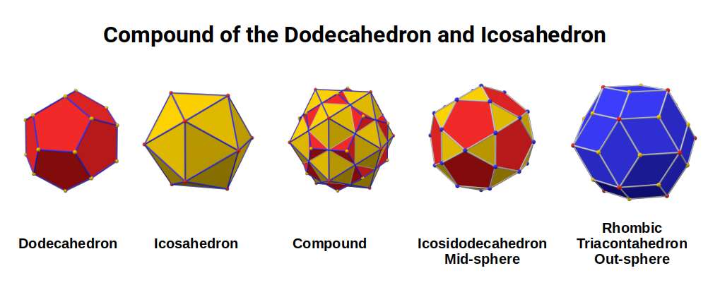
The transition from 28 to 30 neutrons occurs from Chromium (24) to Manganese (25). Geometrically, two Rhombic Dodecahedra transform into a single Icosidodecahedron. The Cuboctahedron with a side of 1.154 can collapse into an Icosahedron (out-sphere ~1.1Å, mid-sphere 0.934Å) which can be compounded with a Dodecahedron (out-sphere 1Å). This provides the geometric mechanism by which the 28 neutrons of Chromium can increase to 30 in Manganese.

Manganese (25) has 55 nucleons, which is exactly the number needed to form a larger Cuboctahedron. As the proton count increases to 26 for Iron, the Cuboctahedron can be divided into two, each containing 13 spheres. Both elements exhibit 30 neutrons. As the Cuboctahedron begins to divide, the Deltoid Icositetrahedron with 26 corners takes over as the outer shell geometry — transitioning from the Rhombic Cuboctahedron (24 corners, Chromium's proton count) through the large Cuboctahedral structure of Manganese.

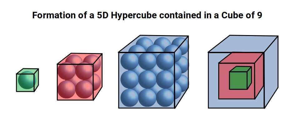
Cobalt (27) has 27 protons — a cube with a side of 3. At the centre of this cubic structure of 27 spheres sits a single sphere surrounded by 26 others, dividing the structure into two, just like the projection of a 4D hypercube. The structure of three nested cubes resembles the shadow projection of a 5D hypercube. The 5D cube has 32 corners, the same as the Rhombic Triacontahedron, and the same as the neutron count of the Cobalt atom.

Iron (26) is by far the most ferromagnetic element on the periodic table, followed by Cobalt (27) and Nickel (28) — the only elements exhibiting ferromagnetism at room temperature. As elements transition from Iron to Cobalt, the radius drops from 1.4Å to 1.35Å, indicating a geometric shift from the Rhombic Cuboctahedral duals to the Snub Cube duals. This arises from the Cuboctahedron (side 1Å) transitioning to a Cuboctahedron (side 1.154Å). During this transition, there is a point where the side-length of the Icosahedron becomes √5-1 (= 2×1÷Φ, the Golden Ratio), producing a side length for the Icosidodecahedron of 1÷Φ.

The mid-sphere of the construction equals 1, which is also the out-sphere of the Icosidodecahedron. Applying this to the nucleus of Iron: when the radius drops to 1.35Å, the Rhombic Triacontahedron forms with an out-sphere of 1. As the mid-sphere of 1 transitions to an out-sphere of 1, the atomic radius collapses. For Nickel, the out-sphere of the Icosidodecahedron becomes 1, unifying with the Icosahedron (side 1.154).

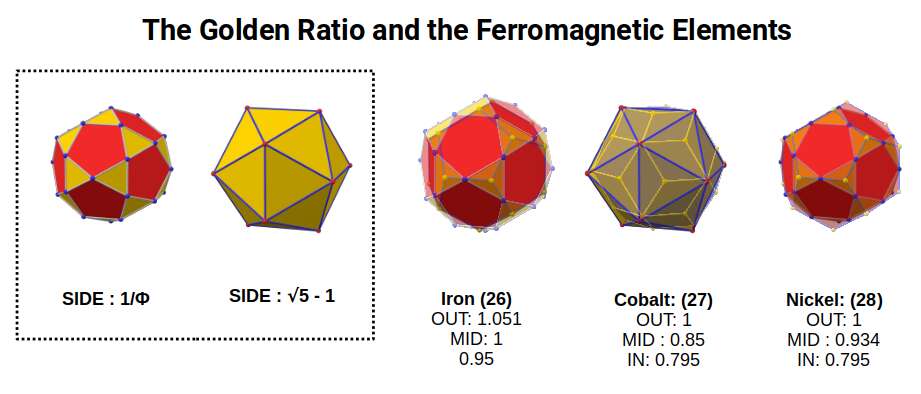
The Golden Ratio can be easily derived from the pentagon. In the case of Iron, the Icosidodecahedron also exhibits a side of 1÷Φ. This produces geometric correlations that extend to much higher dimensions — one key example being the famous E8 geometry from which the Icosidodecahedron can be extracted. Rather than attributing ferromagnetism purely to the electron configuration, this model suggests the real cause lies in the Golden Ratio expressed by the Icosidodecahedron's side lengths and the Deltoid Icositetrahedron formed by the protons.

Why Chromium and Manganese are not ferromagnetic

Traditional theory suggests that the ferromagnetic qualities of Iron, Cobalt, and Nickel are due to these atoms exhibiting large numbers of unpaired D-orbital electrons. This explanation fails on its own terms: Chromium (24) exhibits even more unpaired electrons and is antiferromagnetic. Manganese (25) also has many unpaired electrons yet shows no ferromagnetic properties. The same is true of D-orbital elements in higher shells with equivalent unpaired electron counts. (One other element, Gadolinium, is known for ferromagnetic properties, though it tends to lose its magnetic domains at room temperature. Gadolinium has 64 protons — also a cubic number, 4³.)

The geometric model provides a complete explanation. The fundamental difference between ferromagnetic and antiferromagnetic is the north/south orientation of electron spin within a compound. Chromium always alternates between orientations, whilst Iron's ferromagnetism arises from uniform north-south alignment. When we consider the atom as a 4D structure, this behaviour can be attributed to the nature of 4D rotation — which we suggest is why electrons can only exhibit either UP or DOWN spin.

As Chromium completes the Rhombic Cuboctahedral structure, this 4D rotation unifies in alternating up-down orientation, producing antiferromagnetism. Iron, exhibiting the dual of the Rhombic Cuboctahedron (the Deltoid Icositetrahedron), shows exactly the opposite behaviour — atoms aligning over large areas of a compound to form magnetic domains.

We can now review the full geometric transition from Chromium (24) with its antiferromagnetic qualities, through to the ferromagnetic elements. Iron (26) is the most ferromagnetic element; the transition between opposing magnetic properties is separated by Manganese (25) with its large Cuboctahedral structure, which changes the proton geometry from the Rhombic Cuboctahedron into its dual.

As Cobalt forms, the radius decreases along with the ferromagnetic properties, continuing through to Nickel. All of these elements express either 30 or 32 neutrons (Icosidodecahedron or Rhombic Triacontahedron respectively), inheriting higher 'dimensionality' that we will explore further at the end of this article.

The reason Manganese — with the same neutron structure — does not exhibit ferromagnetic qualities is that a Cuboctahedron can nest spheres perfectly in space, preventing the field from accumulating throughout a compound. In simple terms, the Rhombic Cuboctahedron and Cuboctahedron can produce a uniform honeycomb, whilst the Deltoid and Pentagonal Icositetrahedra and Snub Cube cannot.

The lattice structures of elements are an expansive field in solid-state physics and materials science, well beyond this simplified description. Often, elements that exhibit no ferromagnetic or conductive nature as uniform compounds can begin to express these properties in structures combining more than one atom type. However, as a generalisation, this model offers a geometric explanation for the ferromagnetic (and antiferromagnetic) properties of these elements that explains why other atoms with equivalent unpaired electrons according to present theory are not magnetic.

Copper and Conductivity

The final four elements of the D-orbital set all share the same radius of 1.35Å. Of these, the first two — Cobalt (27) and Nickel (28) — exhibit ferromagnetic qualities. From Nickel (28) to Copper (29) there is a large jump in the total neutron count. Copper comes in two isotopes with 63 or 65 nucleons (~70%/30% ratio), averaging roughly 64 — a cubic number (4³). Zinc (30) exhibits three main isotopes ranging from 64 to 68 nucleons.

Copper is the second most conductive element on the periodic table after Silver (47), and the third most conductive is Gold (79). Each appears in the same location in the three stable D-orbital blocks and each exhibits only a single electron in its outer shell. This single S-orbital is often attributed as the reason for conductivity. However, many other D-orbital elements also exhibit a single outer S-orbital electron (particularly in the 2nd D-orbital set) without equivalent conductivity. A more complete solution is found in Bloch's theorem, which examines conductivity from a wave perspective rather than the electron particle model.

The Dual of the Snub Cube — the Pentagonal Icositetrahedron — has 38 corners. Subtracting this from the nucleon counts of the Copper isotopes (63 and 65) leaves 25 and 27, the proton counts of Manganese (25) and Cobalt (27).

As noted previously, the Cuboctahedron has 12 corners but nests 13 spheres. Therefore 13+12=25 produces the geometry of two nested Cuboctahedra. The 2nd Copper isotope with two more neutrons increases this to 27 — the corners of a dual compound of a Cuboctahedron and Rhombic Dodecahedron. Comparing this geometric configuration to Iron, the most ferromagnetic element, the differences are 7 and 9 respectively. Geometrically, 7 forms the corners of an Octahedron with an additional unit at the centre (6+1), and a body-centred Cube (8+1).

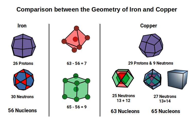
The Octahedron and Cube are both found within the construction of the Deltoid and Pentagonal Icositetrahedra. As each transforms from its dual, the Octahedron increases in size, pushing through the square faces on the x, y, and z axes, whilst the eight corners defining the cube collapse. This affects the overall Rhombic Cuboctahedral D-orbital model. In Iron, the Deltoid Icositetrahedron produces an in-sphere of 1.22Å (the out-sphere of the √2 Cube), whilst the Octahedron expands to an out-sphere of ~√2Å with a mid-sphere of 1Å and side length 2 — forming the perfect relationship to produce a compound of the Cube and Octahedron, the template for the Rhombic Dodecahedron.

The Pentagonal Icositetrahedron of Copper reduces the Octahedron, giving it a smaller mid-sphere of 0.94Å. An Octahedron with its corner caps removed (dividing each side into three) creates a Truncated Octahedron with an out-sphere of 1Å. The dual of the Truncated Octahedron, the Tetrakis Hexahedron, nested around it also produces an out-sphere of 1.22Å — matching the √2 Cube.

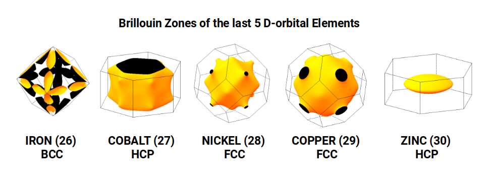
The Truncated Octahedron is recognised as an important polyhedron in the production of conductive fields. These are called Brillouin Zones — derived from the 'reciprocal' space (k-space) of elemental compounds. Each element exhibits a different Brillouin Zone, partly dependent on the compound's crystal structure geometry. Iron exhibits an Octahedral Brillouin Zone, whereas Copper, Silver, and Gold all exhibit Truncated Octahedral zones. In solid-state physics, these are recognised as key reasons for the electromagnetic properties of different elements. Our article on the geometry of Brillouin Zones covers this in much greater detail.

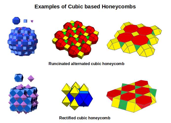
The nature of Brillouin Zones is highly influenced by the compound lattice type. Iron exhibits a Body Centred Cubic (BCC) formation — nine sites with eight at the corners of a Cube and one at the centre. Copper exhibits a Face Centred Cubic (FCC) formation — similar but with the central point removed and additional points placed at the centre of each face, forming a nested Cube and Octahedron. The third type found in D-orbital elements is the Hexagonal Close Packing (HCP) configuration, formed of hexagonal rings of seven points, indicative of the Cuboctahedron. When we compare these atomic crystal structures to a 4D hypercube passing through a 3D plane along its various axes, each produces a close match to the three different types.

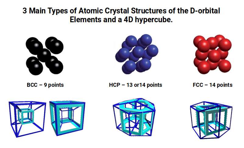
This correlation between 3D and 4D space offers a unique perspective on the crystal geometry of D-orbital elements, producing a foundation that can offer new insight into the energetic structures of various compounds and solids.

Notice that the final element, Zinc (30), exhibits an HCP formation, which changes the Brillouin Zone shape and is the main reason it is not a particularly good conductor. Therefore, whilst both Copper and Zinc are attributed Pentagonal Icositetrahedron geometry, when the compound forms, the orientation of the 4D cube shifts, preventing the electron wave from propagating as effectively. Zinc (30 protons) is renowned for its ability to resist oxidisation and is often used to galvanise metal. Its third stable isotope (30 protons, 38 neutrons) forms the corners of the Icosidodecahedron and Pentagonal Icositetrahedron — after which the D-orbital elements give way to the next P-orbital set.

The Compound of the Extended Jitterbug

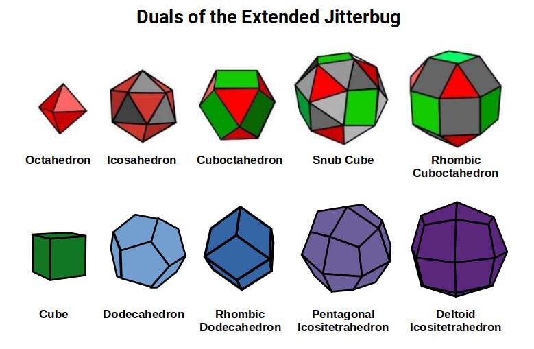
In this article we have examined the nature of the atom in great detail through the principles of geometry. At its heart lies the Extended Jitterbug, producing the Rhombic Cuboctahedral model of 4D hypercubic space. Each of the five solids in the Jitterbug's construction has a dual, always present at any stage. As the Rhombic Cuboctahedron completes with Chromium (24), so the dual begins to emerge up to Iron (26), after which the radius of the atom collapses into the Snub Cube. As the D-orbitals begin to complete, so the Snub Cube gives way to its dual for the final two D-orbital elements, after which the next P-orbitals begin to form.

When we examine the duals of the Extended Jitterbug geometries, we find the Cuboctahedron transforms into the Rhombic Dodecahedron (the template for 4D hypercubic space), formed from a compound of a Cube and Octahedron. The Icosahedron and Dodecahedron duals are also present, producing a total of ten different polyhedra in the set.

These duals can be compounded to create a set of solids from the out and mid-sphere intersection. In the Cube–Octahedron example, the compound creates a Rhombic Dodecahedron from the unification of corners; removing the corner caps creates the Cuboctahedron. Therefore, these duals appear at both the start and the centre of the Jitterbug transformation.

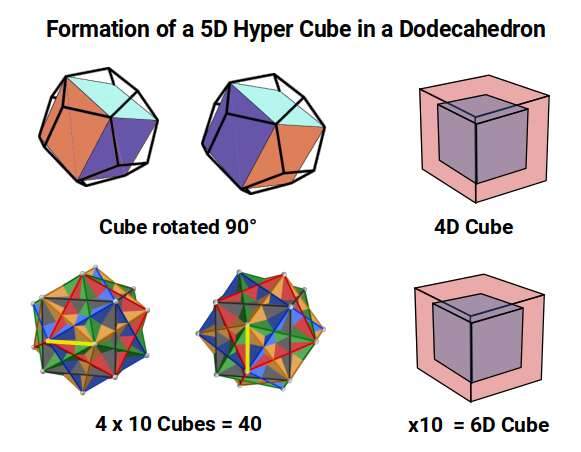
When we examine the full set, many of the geometries assigned to the D-orbital elements reappear. Icosahedral duals produce the 30 and 32 corners found in the neutron counts of elements 25 to 28, whilst the 28-neutron count of elements 23 and 24 is found in the Rhombic Dodecahedron. The Rhombic Dodecahedron provides the template for the 4D Hypercube, whilst the Rhombic Triacontahedron forms the template for the 6D Hypercube. Completing the dimensional picture, the Dodecahedron represents the 5D Hypercube: a Cube can be nested inside a Dodecahedron in five different orientations, and each can also be rotated in two 90° positions, producing a total of 40 Cubes — the number of cubic cells needed to form a 5D Hypercube.

This completes a geometric process that sees the transformation of cubic space into 4D through the Rhombic Dodecahedron, into 5D through the Dodecahedron, and into 6D through the Rhombic Triacontahedron — aligned with the order of compound solids in the first half of the Extended Jitterbug.

In the final set of solids, the Snub Cube and Rhombic Cuboctahedron duals define the radius of the D-orbital elements. These produce compounds with mid and in-spheres that, as far as we are aware, currently lack classification. The mid-sphere of the Snub Cube compound exhibits pentagonal faces similar to the Icosidodecahedron, but also includes six square faces on the x, y, and z axes where the Octahedron corners are found.

Whilst the Jitterbug was first proposed by Buckminster Fuller as a potential correlate to atomic structure, by extending the concept to incorporate the Snub Cube and Rhombic Cuboctahedron, we have produced a valuable geometric tool that can accurately define the radii of the D-orbital elements (and also the P and F-orbital types) to a much greater degree than the Bohr Model. It also begins to offer a new way of modelling the evolution of electromagnetic waves and other properties of atomic lattice structures in more detail than the Schrödinger equations, which model energetic waves only in 3D space.

More importantly, this model suggests that the atom is an integrated multidimensional structure, whereby protons and neutrons form geometries that fundamentally change the properties and behaviour of each element. This holistic approach is the first of its kind to integrate the atomic nucleus, the electron cloud, and the subtle interactions between compounds of different elements.

Conclusion

This article set out to demonstrate a single thesis: that the 1st D-orbital set maps geometrically onto the Cuboctahedron and Rhombic Cuboctahedron, and that this geometry — rather than probabilistic electron shielding — explains the key anomalies of the transition metals. The evidence presented supports that thesis across three distinct tests.

Atomic radii. The experimentally determined radii of all ten 1st D-orbital elements cluster around exactly two values: 1.4Å and 1.35Å. The Bohr model cannot predict these values for D-orbital elements. The Extended Jitterbug predicts them precisely: 1.4Å corresponds to the out-sphere of the Rhombic Cuboctahedron, and 1.35Å corresponds to the out-sphere of the Snub Cube. Every switch between these two radii across the set corresponds to a geometric transition in the Extended Jitterbug sequence.

Aufbau anomalies. Chromium (24) and Copper (29) each 'borrow' an electron from their outer S-orbital to prematurely complete the D-orbital set — a behaviour standard theory attributes to electromagnetic shielding without a precise mathematical derivation. In the geometric model, both anomalies occur at exactly the same condition: a total nucleon count divisible by 13. Chromium has 52 nucleons (4×13); Copper has 65 nucleons (5×13). The nucleus, not the electron cloud, drives the anomaly.

Ferromagnetism. Standard theory attributes the ferromagnetism of Iron, Cobalt and Nickel to their high counts of unpaired electrons — yet Chromium has more unpaired electrons and is antiferromagnetic, and Manganese also has many unpaired electrons with no ferromagnetic properties at all. The geometric model resolves this: Iron's proton geometry forms the Deltoid Icositetrahedron (the dual of the Rhombic Cuboctahedron), which supports the uniform north-south spin alignment required for ferromagnetism. Chromium, completing the Rhombic Cuboctahedron itself, produces alternating spin orientations through its 4D rotational symmetry. Manganese, with its large space-filling Cuboctahedral structure, prevents the magnetic field from accumulating across a compound. The Golden Ratio appears naturally in the nuclear geometry of Iron at the point of the transition — an observation that connects this model to the broader mathematics of higher-dimensional polytopes.

Together, these three results establish that the atom in this region of the periodic table is not adequately described by a probabilistic electron cloud alone. The geometry of the nucleus — the specific polyhedra formed by proton and neutron counts — directly governs the observable chemistry. This is the central claim of Atomic Geometry and the sub-disciplines of Geo-quantum Mechanics and Geo-nuclear Physics.

The theory of Atomic Geometry and its subdisciplines are still in their infancy. Yet the initial correlations to observed phenomena provide a much closer match than any other model thus far. Graphing the orbital radii of the geometric model against the experimentally determined radii and the Bohr Model predictions yields a result far more consistent with experimental data — making Atomic Geometry the most accurate predictive model of the atom for this set of elements currently available.

The implications extend well beyond the periodic table. Understanding the precise geometric conditions for ferromagnetism and conductivity has direct applications in materials science — particularly in the development of new compounds for quantum computing, renewable energy storage, and high-temperature superconductors. By replacing vague probabilistic shielding arguments with exact geometric constraints, this framework gives researchers a principled basis for predicting the electromagnetic behaviour of novel transition metal compounds before synthesising them.

In Part 2, we extend this analysis to the 2nd and 3rd D-orbital sets, examine the mystery of Technetium (43) and its position at the exact midpoint of the stable elements, and explore how the same Extended Jitterbug framework scales across the broader structure of the periodic table.

FAQ

Why are Iron, Cobalt and Nickel ferromagnetic but not other D-orbital elements like Chromium or Manganese?

The ferromagnetic properties of Iron (26), Cobalt (27) and Nickel (28) arise from the geometric structure of their atomic nuclei. Their neutron counts correspond to the corners of the Icosidodecahedron and Rhombic Triacontahedron — solids derived from the Golden Ratio — which produce a nuclear geometry that aligns electron spin domains uniformly across a compound. Chromium (24), by contrast, completes the Rhombic Cuboctahedron, whose 4D rotational symmetry causes alternating spin orientations (antiferromagnetism). Manganese (25) forms a large Cuboctahedral structure that tiles space perfectly, preventing the field from accumulating.

What are the Aufbau Anomalies and why do they occur at Chromium and Copper?

The Aufbau Principle predicts that electrons fill orbitals in a regular sequence, but Chromium (24) and Copper (29) each 'borrow' an electron from their outer S-orbital to complete a D-orbital configuration prematurely. In Atomic Geometry, both anomalies occur when the nucleon count is divisible by 13 — the number of spheres that nest perfectly inside a Cuboctahedron. Chromium has 52 nucleons (4×13) and Copper has 65 nucleons (5×13). The geometry of the nucleus drives the anomaly, not a mysterious electromagnetic interaction.

What is the Extended Jitterbug and how does it relate to D-orbitals?

The Jitterbug Transformation, first described by Buckminster Fuller, shows how an Octahedron can transform into a Cuboctahedron by opening its faces. Atomic Geometry extends this sequence to include the Snub Cube and Rhombic Cuboctahedron, forming the 'Extended Jitterbug'. The five solids in this sequence map directly onto the two geometric types of D-orbital: the three cubic cross-shaped orbitals correspond to the Cuboctahedron, and the two torus-type orbitals correspond to the Rhombic Cuboctahedron. The transition between these solids accurately predicts the two main atomic radii (1.35Å and 1.4Å) found across all 1st D-orbital elements.

Why is element 43 (Technetium) radioactive?

Element 43 (Technetium) appears at the exact midpoint of the three stable D-orbital blocks, with 34 stable elements on each side from hydrogen to bismuth. Its radioactivity is examined in detail in the second part of this series on D-orbital geometry.