
The 3rd set of D-orbitals are the last to form stable elements. The geometric explanation revels a 6D structure which terminates as the end of the Metatron’s cube template.
Overview
Previously, we have discussed the nature of the 1st and 2nd D-orbital set revealing a geometric model that based on a Rhombic Cuboctahedron, and Truncated Cube. This reveals a 4D and 5D hypercubic nature to the orbital forms. Halfway through the 2nd D-orbital set, the geometry transitions into the phi ratio, forming an Icosidodecahedral formation, which causes the decay of the radioactive, Technetium (element 43). After this, the d-orbitals shift back towards the octahedral form of the Triakis Octahedron, (dual of the Truncated Cube).
This 3rd part on the D-orbitals reveals how the model extends into the 6th dimension through the Great Rhombic Cuboctahedron, ending in the Triacontahedron, which is the template for the 6D hypercube. The shadow projection of these solids is found as the Metatron’s Cube completes the shadow projection of the completed set of 5 Platonic Solids, which revels why reality is limited to only 81 stable elements.
KEy Points
-
Geometric theory can explain the quantised states of the atom
-
The atom contract due to the nature of the golden ratio. The radius of the final stable element (83) is 1.6Å
-
The Great Rhombicuboctahedron can be used to model the final set of D-orbitals
3rd D-orbital set
The 3rd D-orbital set runs from elements 70 to 80, and form in the 5th shell, directly after the F-orbitals complete the 4th shell. The first element, lutetium (70) exhibits a radius of 1.75Å, the same as the preceding F-orbitals. Subsequently, the elements decrease in radius, falling to 1.55Å for Hafnium (71), 1.45Å for Tantalum (72), and then Tungsten (73) and Rhenium (74) both have radii of 1.35Å. This completes the first half of the D-orbital set.
Similar to the previous D-orbitals, the 6th element, Osmium (76), exhibits a smaller radius than other D-orbital elements of 1.3Å. After this, the orbital radius increases to 1.35Å for the next three elements. The final element, Mercury (80), exhibits a slightly anomalous radius of 1.5Å. The 8th and 9th elements, Platinum (78) and Gold (79), both exhibit anomalies in their electron configuration, with only a single S-orbital in the outermost shell.
Up electrons
|
Element
|
D-orbital
|
S-orbital
|
Radius
|
|---|---|---|---|
|
Lutetium (71)
|
1
|
2
|
1.75
|
|
Hafnium (72)
|
2
|
2
|
1.55
|
|
Tantalum (73)
|
3
|
2
|
1.45
|
|
Tungsten (74)
|
4
|
2
|
1.35
|
|
Rhenium (25)
|
5
|
2
|
1.35
|
Down electrons
|
Element
|
D-orbital
|
S-orbital
|
Radius
|
|---|---|---|---|
|
Osmium (76)
|
6
|
2
|
1.3
|
|
Iridium (77)
|
7
|
2
|
1.35
|
|
Platinum (78)
|
9
|
1
|
1.35
|
|
Gold (79)
|
10
|
1
|
1.35
|
|
Mercury (30)
|
10
|
2
|
1.5
|
Except for Mercury (80), we can map the evolution of these radii through the out, in and mid-sphere, of two Rhombic Triacontahedra. The first is derived from the Icosahedron, with a side length of 2.3Å and the second form an icosahedron with a side of 1.6Å. In our examination of the 2nd D-orbital set, we saw how these lengths are derived from a Cuboctahedron with an out-sphere of 1.15Å, the doubles to 2.3Å as it transitions through the Jitterbug. The second radius of 1.61Å relates to the Gloden Ratio, which appears as the 2nd D-orbital set completes.
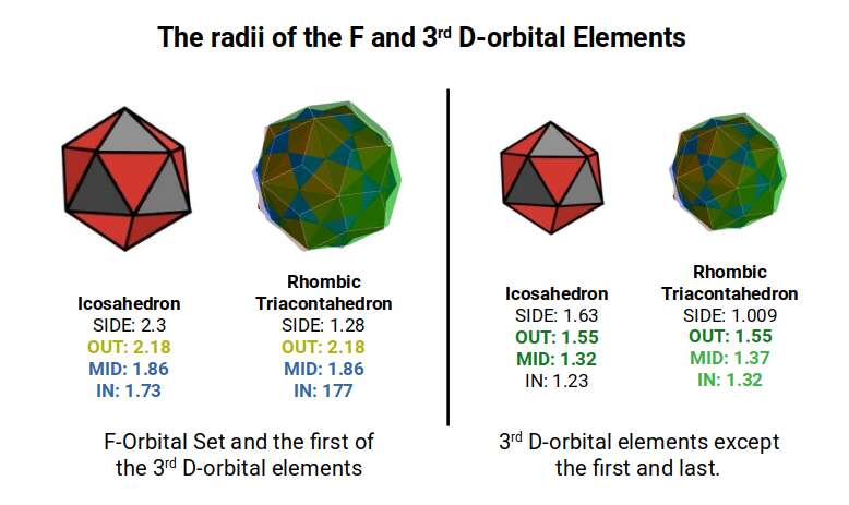
From the perspective of geometry, the final orbitals now centre around the mid-sphere of the smaller Rhombic Triacontahedron. This forms the template for the 6D Hypercube.
As with the previous D-orbital sets, we can see what emerges when we expand a Cuboctahedron through the Dodecahedron transformation. This time as the 4th P-orbital set, Elements 49-54, exhibits a radius of 1.41, or √2. This means that when transformed through the Dodecahedron, the final Cuboctahedron will exhibit a larger side length of 2. Notice this is roughly the same size as the average radius of the 2nd P-orbital set, which begins with a Cuboctahedron with a side of 1. When transformed through the Rhombic Dodecahedron and the Jitterbug, this also produce a new Cuboctahedron with a side length of √2.
The Cuboctahedron (Left) with a side of 1.41 (√2) transforms through nested relationship of the cube, dodecahedron, and icosahedron, which finally expands through the jitterbug into a Cuboctahedron (Right) with sides √2 greater.
We can see that the Cuboctahedron can produce a compound of the Cube and Octahedron, and in doing so define the foundational radii of the 2nd, 3rd, and 4th P-orbitals sets, 1Å, 1.154Å, and 1.41Å respectively. The Dodecahedron that sit around the Cube exhibits a Mid-sphere of 1.61, which represent the largest D-orbital Elements, Scandium (21), and Sliver (47). Whereas the Insphere roughly defines the radius of 1.35Å found in the majority of D-orbitals. The Icosahedron Exhibits an in-sphere of 1.5, which is the radius of Mercury (80) the last D-orbital elements. After this, only 3 more P-orbitals form before the radioactive element begin.
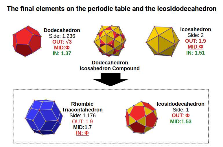
The first, Thallium (81), exhibits a radius of 1.9Å, found in the Outsphere of the Icosahedron. This is followed by Lead (82) which is sometimes quoted as having a radius of 1.8Å or 1.75Å. The latter is found in the out sphere of the Dodecahedron. Finally, the last stable element on the periodic table, Bismuth (83), has a radius of 1.6Å, which is found in the mid-sphere of the Icosahedron and Dodecahedron, the point where the Rhombic Triacontahedron is formed.
As the Icosahedron has a side of 2, its mid-sphere will be the golden ratio (Φ), 1.618. Whereas, the side of the Dodecahedron is 2÷Φ, and the Rhombic Triacontahedron has a side of 1. This means that the atoms on the stable periodic table terminate once at the Phi ratio, in the mid-sphere of the Triacontahedron, which is the template for the 6D Hypercube.
We can compare the Geometric model to the Bohr and Experimental Dataset. As with the other D-orbital elements, the Bohr model overshoots the radii of the D-orbital set. Furthermore, as the 5th P-orbitals form, we find that the Bohr radius drastically undershoot the experimental values.
|
Element
|
Radius
|
Geometric
|
Bohr
|
|---|---|---|---|
|
Lutetium (71)
|
1.75
|
1.73
|
2.17
|
|
Hafnium (72)
|
1.55
|
1.55
|
2.08
|
|
Tantium (73)
|
1.45
|
1.47
|
2
|
|
Tungston (74)
|
1.45
|
1.47
|
1.93
|
|
Rhenium (75)
|
1.35
|
1.37
|
1.88
|
|
Osmium (76)
|
1.3
|
1.32
|
1.88
|
|
Iridium (77)
|
1.3
|
1.37
|
1.8
|
|
Platinum (77)
|
1.35
|
1.37
|
1.77
|
|
Gold (79)
|
1.35
|
1.37
|
1.74
|
|
Murcury (48)
|
1.5
|
1.5
|
1.71
|
|
Thallium (81)
|
1.9
|
1.9
|
1.56
|
|
Lead (82)
|
1.75
|
1.73
|
1.54
|
|
Bismuth (83)
|
1.6
|
1.618
|
1.35
|
The existing model has no explanation for the sudden increase in the these last P-orbital sets, nor why only 3 out of 6 should be stable. In the final elements, we find there are a total of 5 electrons in the outmost shell. This matches the pentagonal geometries formed but the Icosahedron and Dodecahedron. Similarly, we find the 5th element on the 2nd D-orbital set is unstable, as the set transitions from 4D to 5D, only this time the D-orbital structure moves into the 6th dimension.
The Rhombic Triacontahedron and the Icosidodecahedron.
The Rhombic Triacontahedron defines the blueprint for the 6D hypercube, in the same way that the Rhombic Dodecahedron forms the blueprint of the 4th dimensional cube. Whilst is can be created by compounding the dodecahedron and Icosahedron, it can also be formed through a similar process to the jitterbug. In this case, each square face of the cube is divided in half, and expanded to create two new triangular faces. This can be accomplished in exactly two different orientation, with the split running through the horizontal or vertical of the cubes face. Similarly, the new vertex that is created between the two triangles is also orientated at 90°, mirroring the orientations found in the Star-Dodecahedron. This in turn gives the Rhombic Triacontahedron two distinct possibilities in terms of orientation.
A cube with a side length of 2 has an in-sphere of 1, and a mid-sphere of 1.41, which is the radius of the 2nd and 4th P-orbital set. When transformed into a Rhombic Triacontahedron each side is halved in length. This produces a Triacontahedron with an out-sphere of 1.45, and mid-sphere of 1.37. These two radii are found to predominate the D-orbital sets, beginning with, iron (26). The entire second half of the 1st D-orbitals, all conform to a radius of 1.35Å. The start and end of the 2nd D-orbital set sees many of the elements conform to a radius of 1.35Å, or 1.45Å. In the 3rd D-orbital set, the radius of the cube, 1.41Å, is missing from the set. The elements fall from 1.45Å to a radius of 1.35Å. What we can begin to perceive is that the 6D cube begins to form around this particular area, that is also where the D-orbital sets are generally composed.
As the Triacontahedron comprises a compound of an Icosahedron and Dodecahedron, it naturally inherits the pentagonal geometries, which exhibit the golden ratio. If its side length is 1 the out-sphere that encompasses it will be phi. The difference between the out and mid-sphere is √1.25, which, when 0.5 is added, also equals Φ. Just as the Icosahedron exhibits a pentagonal prismal mid-section, the same is inherited by the Rhombic Triacontahedron. However, due to the intersection of the Dodecahedron, a second pentagonal plain can be found internally. These two types of pentagon exhibit the side length of the Icosahedron and Dodecahedron, which when compounded are in a 1:Φ Ratio
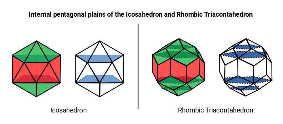
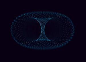
The Theory of Atomic Geometry suggested the Icosahedron forms a double torus found in the F-orbital set, denoted by the fact that it is comprised a pentagonal prism as its centre. The Rhombic Triacontahedron extends this notion, adding another layer from the pentagonal sides of the Dodecahedron. Similarly, the final D orbital torus completes a set of 3 torus fields, which can be represented in its structure.
The Rhombic Triacontahedron also has a dual, the Icosidodecahedron. This solid can be formed by truncating the corners of a Dodecahedron or Icosahedron, analogous to the truncation of a Cube or Octahedron that creates the Cuboctahedron.

When we examine the structure of a compound of the Icosahedron and Dodecahedron, generated by the 4th P-orbitals set, We find that the Rhombic Tricontahedron, exhibits an out-sphere of 1.9, the radius of the initial 5th P-orbital element. The Final Element, Bismuth, has a radius of Φ, Which is found throughout the set, But also as the out-sphere of the Icosidodecahedron. Notice that this polyhedron has a side length of 1, exactly half that of the Icosahedron from which it was derived. Its in-sphere has a value of 1.53. This is close to 1.55Å, the experimentally determined radius for many of the D-orbital elements.
The radius of 1.55Å first appears for Zirconium (40), after which the 2nd D-orbital anomalies begin, leading to the instability of Technetium (43). As this set transitions into the 4th P-orbitals, the radius of Silver (47), 1.6Å, Cadmium (48), 1.55Å, and the first P-orbital element, Indium (49) are also found.
Both the Icosidodecahedron, and Rhombic Triacontahedron, transformed from the cube previously, both exhibit the same side length of 1. Between them, we are able to define the radii of the majority of D-orbital radii, as well as many of the S and P-orbital elements.
There is also a relationship between the Icosidodecahedron, and Icosahedron and Octahedron. An Octahedron can be positioned inside an Icosahedron so that its corner touch the mid-point of 6 it edges. As the Octahedron grows in size, so each of its corners push outwards. Inside the Icosahedron, we find 3 golden rectangles can be composed with a side length ratio of 1:Φ. The longer side corresponds to the diagonal across the internal pentagram.
As the Icosahedron has 30 sides, 5 Octahedra can be nests in 5 different orientations, just like the 5-Cube in the Dodecahedron. If the Octahedra is expanded in size, is corners distorts the shape of the Icosahedron, transforming it into an Icosidodecahedron. In doing so, the internal planes are transformed into 3 golden cubes with a ratio of 1:Φ:Φ². As there are five possible orientations for the Octahedron, this means there are also 5 types Icosidodecahedra that can be created from this transformation.
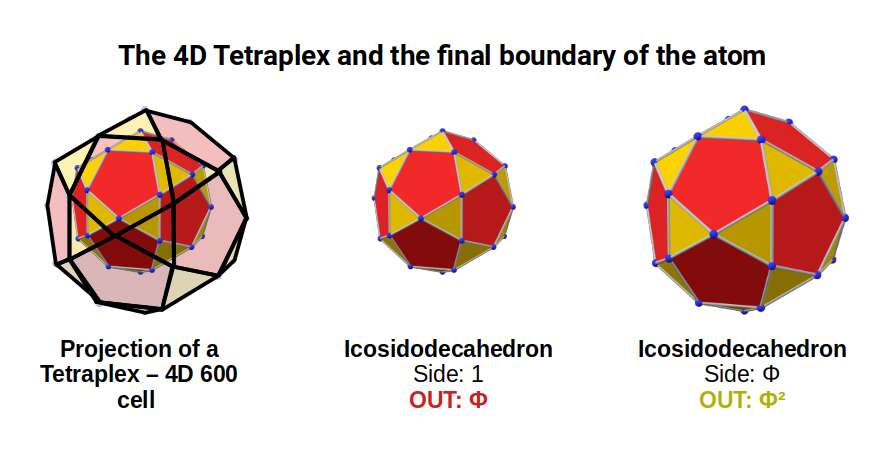
The Icosidodecahedron has recently been recognised being able to represent the E8 Geometry. This multidimensional approach to the atom translates the notions of string theory into Euclidean geometry. The E8 Polytope is an 8th dimensional object, with 240 vertices. This can be projected in 4D as a two 600-cells, called the Tetraplex. Based on the Icosahedron, this 4D polytope is made of tetrahedral cells, and has 120 vertices, exactly. When two combine, the number of vertices doubles, producing the E8 form that is found at the heart of enquiry in the E8 theory.
The Tetraplex is a 4D object, which, like the 4D cube, can be constructed by two nested polyhedra. This can be best applied to a pair of nested Icosidodecahedra. By adjusting some of the vectors to be in golden proportion to the others, each form can be separated by a distance of Φ.
Rotation of the 4D 600-cell
600-cell Projected as 2 Icosidodecahedra
Half a 600-Cell forms the Icosidodecahedra
Each Icosidodecahedra exhibits 30 corner point, which is the number of D-orbital electrons across the 3 shells. Each point is therefore connected to each other through the golden ratio. In the model of half a 600-cell, the mid-point of each pentagonal face has a small protruding point. In higher dimensions, these connected to the second half of the form.
Returning to our geometric model of the atom, we found that an Icosidodecahedron with a side of 1 produces an out-sphere of Φ, and a mid-sphere of 1.53. Previously, we associated these values with the radii formed at the end of the 2nd set of D-orbitals leading onto the 4th P-orbitals set up to the noble gas, Xenon (54). After this, Caesium (55), exhibits the first S-orbital in the 6th shell. This element has a radius of 2.6Å, the largest of any on the periodic table, and is very close to the value 2.618, or Φ². As the 5th P-orbitals begin to fill this shell, only 3 electron form elements, brining the total to 5, (3P and 2S-orbitals). At this point, the radius falls, with Bismuth (83), exhibiting a radius of 1.6, or Φ. Therefore, Caesium (55) that starts to fill the shell 6th shell, and Bismuth (83) that end it, exhibits a Φ relationship, which is perfectly expressed by the projection of a Tetraplex through two nested Icosidodedahedra.
This notion of phi which creates the Golden Ratio is popular in the teachings of Sacred Geometry. But what is not so often recognises is the phi has a sibling called the Sliver Ratio, which also produces a 6D hypercubic modle of the atom.
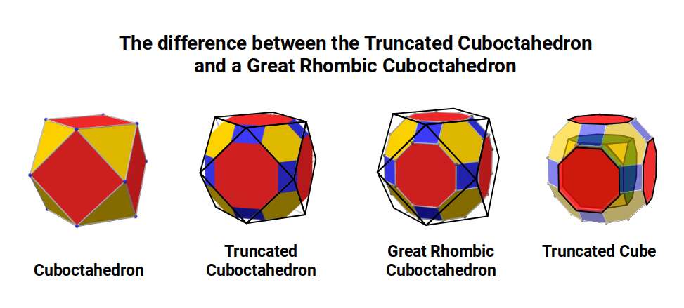
The The great Rhombic Cuboacthedron
The Truncated Cube has a larger brother called the Great Rhombic Cuboctahedron. By moving the Octagonal faces away from the centre, the space between each one becomes sufficient to add a square between each one. At this point, the corners become composed of hexagons, instead of the Triangular faces found in the Rhombic Cuboctahedron.
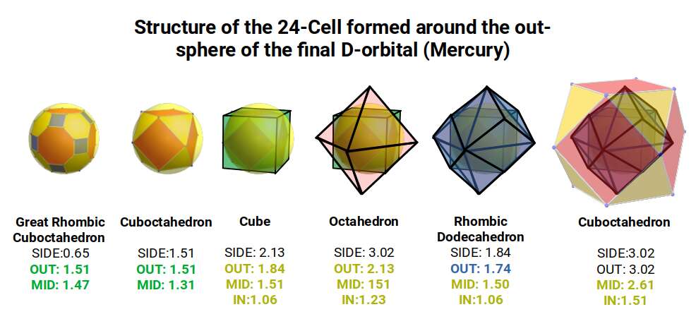
In our Geometric model of the atom, the Truncated Cube appears in the 2nd D-orbital shell, producing the slightly enlarged radius of 1.47Å. Around this we can place a Great Rhombic Cuboctahedron, whereby its mid-sphere meets the out-sphere of the Truncated Cube. This produces a slightly larger out-sphere of 1.51, which is almost exactly the radius of Mercury (80). Notice that the preceding elements all have a radius of 1.35Å, found in the mid-sphere of the Rhombic Triacontahedron. Once the set complete, there is a large jump in radius to 1.5Å, just as the last D-orbital completes. The radius of the out-sphere of the truncated cube, happen to appear only once, at the 3rd element, Tantalum (73), just as the 3 cross shaped D-orbitals form. Therefore, the mid and out-sphere of the Great Rhombic Cuboctahedron appears in the both the 3rd and 10th shell.
Around the Great Rhombic Cuboctahedron, we can place a Cuboctahedron, so that the out-and mid-spheres of each solid align. The Cuboctahedron produces a new out-sphere of 1.74, which is extremely close to the radius of the smaller F-orbitals elements, 1.75Å. In Atomic Geometry, we represent the 4 hexagonal shaped F-orbitals within the structure of the Cuboctahedron.
Alternatively, we can align the out-sphere of the Great Rhombic Cuboctahedron with the in-sphere of a cube. This produces a mid and out-sphere of 2.13 and 2.61. This equates the radius of the last pair of stable S-orbitals, Caesium (55), radius 2.6, and Barium 2.15Å, that form the the 6th shell.
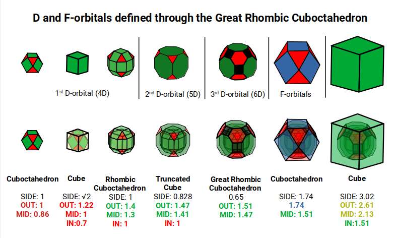
This geometric model expresses a cubic perspective of the D-orbital sets. If we include the Snub Cube with an Out-sphere of 1.35, we can see that all the D-orbital radii are expressed in this model. The smaller Geometries to the left of the set, also provide the radius of many of the 1st P-orbital elements (red). As the geometries build into the 2nd D-orbital set, we find the Truncated Cube introduces the new slightly larger radius of 1.47. Finally, as the 3rd set of D-orbitals complete, we find Mercury, which is the only D-orbital element with a radius of 1.5Å. This model expresses the nature of the hypercube as it expanding through dimensional space. The first D-orbital set contains two cubes, side length 1 and √2, indicative of a 4D hypercube. The Truncated Cube adds another layer to this, producing 3 Cubes, as found in a 5D hypercube. The final layer is produced by the Great rhombic Cuboctahedron, which adds a 4th cube to the set, completing the model of a 6D Hypercube. This final boundary is also expressed as the Rhombic Triacontahedron, That forms the blueprint for the 6D cube, in the same way the Rhombic Dodecahedron produces the 4D hyper cubic template. Thus, through the 6th dimension of the cube, the D-orbitals complete.
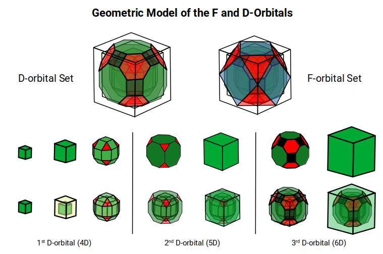
Notice that in the model above, there are 4 cubes indicative of a stereographic projection of a 6D hyper cube. Notice that in the 1st D-orbital set, two cubes are found with a side of 1, and √2. This 4D cubic structure is orientated by the Rhombic Cuboctahedron. The truncated cube is found in the 2nd D-orbital set, which can topologically transform into the Icosidodecahedron, to produce the 5D hyper cubic arrangement inside the Dodecahedron.
The final D-orbital set is represented by the Great Rhombic Cuboctahedron. This has a special relationship to the Rhombic Cuboctahedron. 12 cubes can be placed on the inside of the square faces of the Great rhombic Cuboctahedron, which align perfectly with the square faces of the Rhombic Cuboctahedron. This produces a uniform distance between the polyhedra and its side length, i.e. it is a projection of higher dimensional space of a uniform polytope.
With a side length of 1, the Rhombic Cuboctahedron exhibits an octagonal mid-section that measure √2+1, (the silver ratio), between opposite edges. Adding cubes to either the top or bottom section extends this distance to √2+2, when viewed from above. This is dues to the 45° incline of the attached cube. When the mid-section is extended in the same manner, the distance between edges increase to √2+3. This provides us with an interesting extension of the silver ratio, based on the numbers 1, 2, and 3, as the cube expands into higher dimensional space.
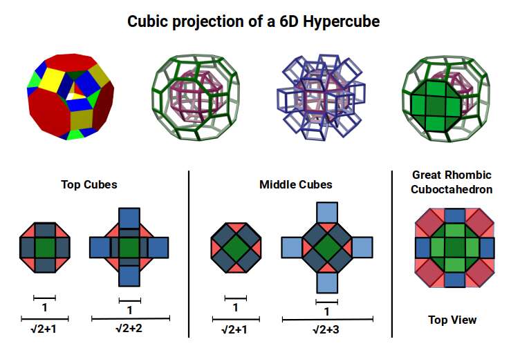
A 6D hypercube of formed of 12 5D hyper cubic faces. This is the same number of cubes added to the faces of the Rhombic Cuboctahedron. If we examine the structure of this cell, we find it consists of two cubes, separated by a gap. The outer cube is extruded from the surface of the Rhombic Cuboctahedron, whilst the other is form from the small cube at the centre, which when exploded in space produces the Rhombic Cuboctahedron. A 3rd Cube can be added to the inside of the Rhombic Cuboctahedron, filling the space between the two. This will either overlap the cube at the centre or when attached to the face of the centre cube will overspill into above the surface of the Rhombic Cuboctahedron. In either state, the ratio of 1:√2-1 is maintained. This is the Silver ratio, which can also be expressed as √2±1. This cubic cell is therefore comprised of 3 cubes, which is indicative of a 5D cube, and is governed by the Silver ratio. A 6D cube exhibits 12 of the 5D cells in its structure, which is the same number found between the unification of the Rhombic cuboctahedron and its bigger brother, the Great Rhombic Cuboctahedron.
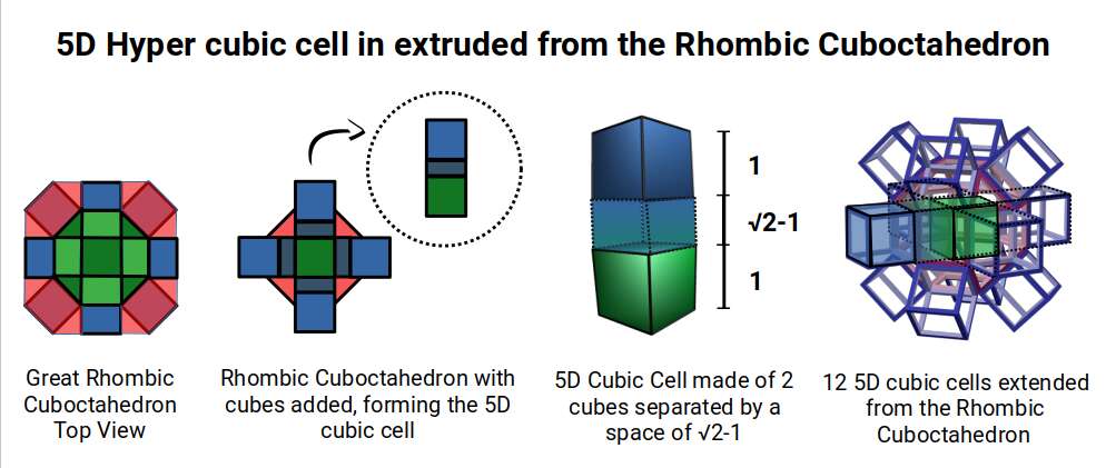
The model of a 6D Cube leaves space above the octagonal faces of the Great Rhombic Cuboctahedron. These can be filled with 6 more Rhombic Cuboctahedra, aligned on the x, y, and z axis. Once complete, we find that the remaining square faces, where the 5D cubic cells were formed, can be filled with another 12 Rhombic Cuboctahedra, brining the total in the set to 19, including the one at the centre of the construct.
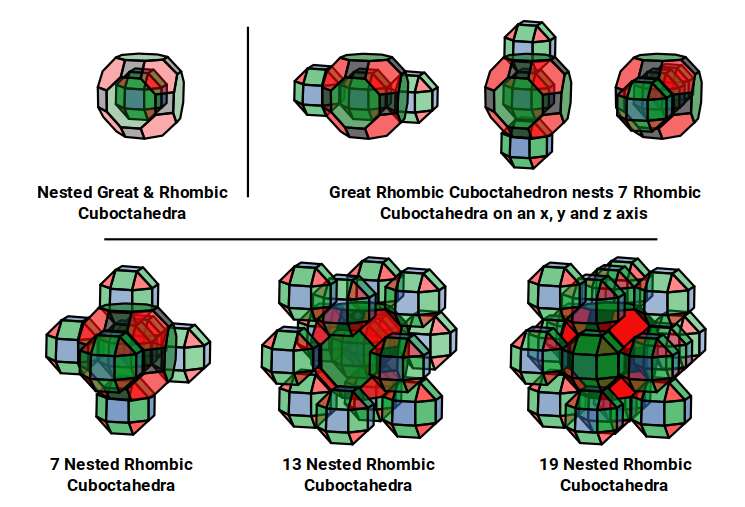
When we separate out these two types of arrangements, we find that they exhibit an Octahedral and Cuboctahedral structure. This matches the geometric arrangement of the D, (and even P), orbital sets. The Octahedral confirmation, can be expanded by adding more Great Rhombic Cuboctahedra to each of the 6 external Rhombic Cuboctahedra. This pattern can be extended indefinitely, leaving small cubic spaces where the 5D cells appear. The same cannot be said of the Cuboctahedral structure. These attach to the outer square faces of the Great Rhombic Cuboctahedron, which prevents the expansion of this set into infinity. What we can recognise is the fractal structure, which could expand indefinitely, is limited to by the Cuboctahedral arrangement. Similarly, there are no stable D-orbital elements beyond the 3rd set, as it is limited to the 6th Dimension, due to its Cuboctahedral nature.
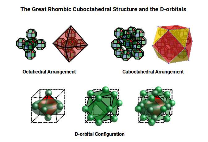
The Octahedral P-orbitals and Cuboctahedral D-orbital Geometries are further distinguished by replacing the Rhombic Cuboctahedra with 6 Truncated Cubes (5D Hypercubes), These fall over the x, y and z axis, representative of the P-orbitals sets. Upon the hexagonal faces of the Great Rhombic Cuboctahedron, Truncated Tetrahedra can be placed. This produces new spaces for a set of 12 more Great Rhombic Cuboctahedra, orientated like the D-orbitals. Interestingly, the F-orbitals contain two star-tetrahedral orbitals, which in the same orientation as the Truncated Tetrahedra. This configuration can be expanded through both an Octahedral and Cubic, similar to the Rhombic Dodecahedron, filling 3D space uniformly, into infinity.
The Light Boundary
When considering the 6D construct produced by the Great Rhombic Cuboctahedron, we notice the side lengths remain consistent throughout the structure. This is different to the D-orbital model presented, where the unification of the mid-spheres of each solid produces a decreed in the side of each subsequent polyhedra. The Rhombic Cuboctahedron is based on a side of 1, which is exploded from a cube with the same edge length. However, he Truncated Cube is derived from a Cube with a side length of 2, giving is a side of 0.828, or √8-2. Note that this is double the value of the silver ratio, √2-1, and so still exhibits the same qualities. The Great Rhombic Cuboctahedron has a side of 0.65, which is close to 2÷3, (0.666…).
When first originally rediscovered by Johannes Kepler, he originally called the Great Rhombic Cuboctahedron the ‘Truncated Cuboctahedron’. However, due to the nature of the Silver Ratio, found in the octagon, and the triangular faces of the Cuboctahedron, this procedure will elongate the square faces formed on the Great Rhombic Cuboctahedron. Therefore, the only correct geometric principle to form this polyhedron is to explode the faces of the truncated cube. Therefore, a Great Rhombic Cuboctahedron will have a side length that is between the longer and shorter sides of the Truncated Cuboctahedron.
We can call this the compressed model, as the difference between the sizes of the Rhombic Cuboctahedron, Truncated cube and Great Rhombic Cuboctahedron a closely spaced together. This is because the Truncated Cube as derived from a cube with a side of 2.
We can also produce a model whereby these 3 polyhedra exhibit the same side length, as presented in our explanation of 6D hyper cubic space. The 1st D-orbital set, up to the Rhombic Cuboctahedron, remains the same. After this, the Truncated Cube is derived from a cube with a side of √2+1. This maintains the size of the Truncated Cubes edges to 1, producing a much larger radius of 1.77, Where the F-orbital elements are found. Note that the F-orbitals appear in this 4th shell.
The Great Rhombic Cuboctahedron with a side of 1 produces a much larger circumference. The Mid-sphere measures 2.26, which is slightly bigger than 2.2Å, the radius of Potassium (19) that appears at the start of the 4th shell. The Out-sphere marks a radius of 2.32, which is close to the radius of Rubidium (37), which appear in the same place in the next shell up. Finally, the radius of Caesium (55), again the first to appear in the 6th shell, is found in the mid-sphere of the Cuboctahedron.
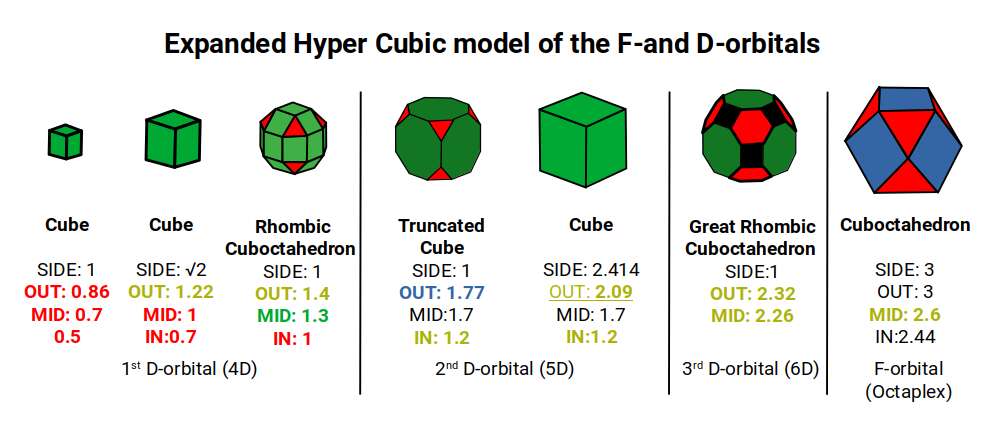
Note that in this model, the value of the side of the Great Rhombic Cuboctahedron is tripled, as if it were truncated from the Cuboctahedron. In fact, the true size of the Cuboctahedron will be marginally larger, as found is the 24-cell compressed model. Notice that when both end at roughly the same point, where the Cuboctahedron with an out-sphere of 3.
We can compare these radii to the experimentally determined results for all S-orbital elements, excluding Helium (1), whose radius of 0.25Å is easily derived from the halving of the first P-orbital radii. When compared to the predictions of the Bohr Model, we can see that this geometric interpretation offers a much closer match to the experimental data.
We can see that the point there both dataset tend to agree is with the radius of Magnesium (1.5Å). After this the Borh model increases in radius, moving away from the experimentally determined values. The geometric modle predicts a slightly larger radius for Strontium, which appears in the same shell as the Orbital set. This has a radius of 2 which is more accurately described by the out-sphere of the Cuboctahedron with the same side length. This was found at the end of the jitterbug transformation of the 4th, P-orbital set.
According to the Bohr Radius, the size of the largest atom, Barium (56), is 2.98Å, which is close to the final out-sphere of the Cuboctahedron created by the both the contracted and extended Hyper cubic model. This value also happens to be close to the speed of light, which is 299,792,458 metres per second. When the meter is scaled to Angstroms, light will take 1 attosecond to travel the radius of the out sphere of the Cuboctahedron, which is 10-18 seconds.
Presently, the limitation of speeds observed by science is 100 attoseconds. Whilst, determining the detailed nature of events at this speed is beyond our present capabilities, we can use this nature of light and produce a scale that denotes the radius of the various atoms and forms a comparison to the geometric nature of space.
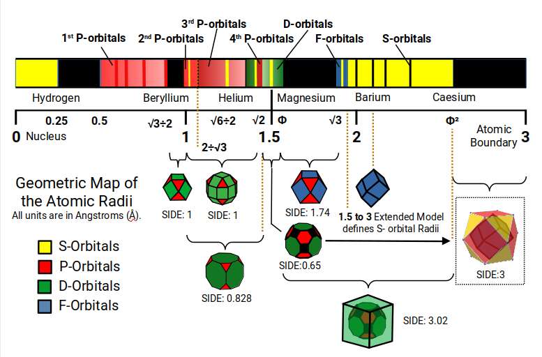
The Scale starts at zero, where the atomic nucleus is found. The smallest Atom, Hydrogen, has a radius of 0.25Å. Then there is a space which again measures 0.25Å, before the next smallest atom is found, Fluorine (9) in the 1st P-orbital set. Notice this form a 1:2 ratio of space. After this, the next smallest atoms are found in the 2nd P-orbital set. The space between the largest of the 1st P-orbitals and the smallest of the 2nd is defined by the mid and out-sphere of the Cuboctahedron with a side of 1.
The 2nd and 3rd P-orbitals overlap, but exhibit a general radius of 1Å and 1.154Å, respectively. Between them site Beryllium (4), with a radius of 1.06Å. When multiplied by the 3rd P-orbital radius (1.154), the result produces the size of the Helium Atom, (√6÷2). From the first 3 P-orbital sets, only Gallium (31) is the largest, with a radius of 1.3Å, due to the face that is appears directly after the first set of D-orbitals form. Aside from this, only two elements, Aluminium (13) and Germanium (32), have a radius of 1.25Å, slightly larger than Helium.
Helium is the first noble gas on the periodic table, inside which we find almost all the first three sets of P-orbital elements. If we multiply its radius again by 1.154Å, it produces the radius of Lithium (1.41Å), or √2. This s-orbital is found at the boundary of the 4th P-orbitals, and most importantly the transition of the D-orbitals from 4D through to 6D. Notice that the D-orbitals appear bunched together, ranging from the smallest, 1.3Å, to the largest, 1.6Å, or Φ. within this area we find the Rhombic Cuboctahedron, Truncated cube, and Great Rhombic Cuboctahedron, which ends with Mercury, and a radius of around 1.5Å. This is also the size of the Magnesium (12) atom is found. This S-orbital elements is key to photosynthesis in plants and is an essential mineral in biology.
If we square the radius of Helium (2), √6÷2Å, then the result is the radius of Magnesium (12), 1.5Å. Notice that this appears at the halfway point on the scale. Like the P-orbitals, only 3 D-orbital elements are larger than 1.6, which appear at the start of end of the D-orbital set. This means that most of the atomic structure is formed in the first half of the scale, similarly that hydrogen divides the first 0.5Å of space into two.
We can multiply 1.5Å by the radius of the 3rd P-orbitals (1.154), to find the smaller radius of the F-orbitals, (1.73Å). Alternatively, we can multiply 1.54 by Φ to produce a radius of 1.87Å, the larger of the two radii. These are separated by two S-orbital elements, Sodium (11), and Calcium (20), as well as the largest D-orbital element, Yttrium (39), that beings the 2nd D-orbital set. Notice that this is where the D-orbital set begins to collapse, where the 5th element in the set, Technetium (43), is radioactive.
Notice that between the smallest F-orbitals (√3Å) and the largest D-orbitals (ΦÅ), there is a space where no atomic radii are found. Just like the space between the 1st and 2nd S-orbitals, this can be found in the mid and out-sphere of a Cuboctahedron. If we employ the extended hyper Cubic Model, the Orbital radius falls approximately where the out-sphere of the Truncated Cube is found, (1.78Å), Close to the radius of Yttrium (39). Only 5 S-orbitals exist beyond the F-orbital band, all of which can be found in the 24-cell formed round the out-sphere of the Great Rhombic Cuboctahedron (6D Hypercube), or the Expanded Hypercubic Model.
THE
Conclusion
What does this tell us about the D-orbitals?
The D-orbitals only consist of three sets, which expand in dimension from the 4D Tesseract to the 6D Hypercube. Phi appears to limit the expansion of the radius, to a maximum of 2.618Å, for Barium (56).
A Geometric approach to the atom
This new approach to the electron cloud can form an accurate prediction of all the stable elements, and is based on the evolution of geometric forms through a series of simple geometric principles.
Carry on Learning
This post form part of our net theory of ATOMIC GEOMETRY, GEOQUANTUM MECHANICS, and GEONUCLEAR PHYSICS. Find out more by browsing the post below.


The 4D Electron Cloud
The electron cloud is normally thought about in terms of the probability of the particle. However, our notion of a 4D Aether dispenses with this notion, returning a sense of normally to atomic physics.
S-orbital Geometry
S-orbitals form the only set of elements occupying a spherical shell. Whilst quantum theory suggests it is ‘only applicable’ to these types of atom, investigation of the atomic radius shows a discrepancy of over 100% for some elements.
2D Orbital Geometry of the Electron Cloud
The 4 types of electron orbital can be mapped to 2D geometry, called the Seed/Flower of Life. This produces a simple geometric pattern that decodes the electron configuration.