Introduction
Pick up a fridge magnet and hold it near your phone screen. You are feeling the same force that guides compass needles, stores data on hard drives, and powers the electric motors in every car. Now plug in a kettle — the copper wires carrying that current are doing something that school physics has never fully explained. Why is copper so uniquely good at the job? Why are iron, cobalt and nickel magnetic when the elements sitting right next to them on the periodic table are not? And why does the answer to both questions involve the same handful of strange mathematical constants?
This article explains all of that — and it does so through geometry.
A crystal is not a random jumble of atoms. It is a precise, repeating lattice — more like a three-dimensional tiling than a pile of sand. The shape each atom adopts within that lattice determines everything: whether the material conducts electricity, whether it attracts a magnet, whether it could one day become a room-temperature superconductor. Brillouin zones are the physicist's way of mapping those shapes into a mathematical space called reciprocal space — think of it as a kind of frequency map of the crystal, showing which directions are easy for electron waves to travel and which are blocked. The zones act a little like lanes on a motorway: some lanes are open, others are closed, and which lane an electron can use depends entirely on the geometry of the lattice around it.
Why does this matter to you? Every semiconductor in your laptop, every magnet in your headphones, and every superconducting material researchers are racing to develop operates according to these rules. Understanding the geometry behind them is not an abstract exercise — it is the foundation of the next generation of materials engineering.
Ferromagnetism and electrical conductivity are not random properties scattered across the periodic table. They arise from the precise geometric structure of the atomic lattice — and Brillouin zones, when interpreted through the lens of Atomic Geometry, make that structure visible.
The standard account of electricity still relies, in many textbooks, on the Drude model: tiny electrons pushed and pulled through a wire like a crowd through a corridor. This model was disproven over a century ago. A more accurate description is Bloch's Theorem, which treats electrons not as particles but as waves propagating through the reciprocal space of a crystal lattice (the mathematical "frequency map" of the crystal described above). The geometric regions that define where these waves can and cannot propagate are the Brillouin zones.
What this article proposes is a significant extension of that framework. Building on the theory of Atomic Geometry — which assigns specific polyhedral forms (three-dimensional geometric shapes) to each element based on its proton and nucleon counts — we find that the geometry of each atom in the first D-orbital set (the row of transition metals from Chromium to Zinc) provides a precise structural explanation for the lattice behaviour of those elements. Iron, Cobalt and Nickel are ferromagnetic because their atomic geometries allow adjacent atoms to rotate in a unified direction. Chromium and Manganese are antiferromagnetic (they resist magnetic alignment by setting neighbouring spins in opposite directions) for the opposite geometric reason. Copper is an exceptional conductor because its geometry — the Pentagonal Icositetrahedron — fits the Brillouin zone structure of the face-centred cubic lattice with a freedom that no other element in the set can match.
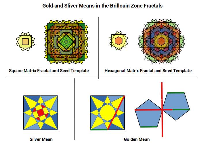
Throughout this investigation, three mathematical constants recur: the Silver Ratio (√2, which appears naturally in the diagonal of a square), the Golden Ratio (Φ ≈ 1.618, the ratio found in pentagons and throughout nature), and the Tribonacci constant (η ≈ 1.839, the three-term cousin of the Fibonacci series). The magnetic field is governed by the Silver Ratio; the electric field by the Golden Ratio. Where the two meet — in the transition from Iron to Copper — the Tribonacci constant provides the geometric bridge.
This is the first model of the atom capable of giving precise geometric reasons for the experimentally observed radii of stable elements, and the first to offer a coherent structural explanation for ferromagnetism, antiferromagnetism, diamagnetism, and electrical conductivity within a single unified framework.
Key takeaways
- Iron, Cobalt, and Nickel are ferromagnetic because their atomic geometries allow adjacent atoms to rotate in the same direction, aligning electron spin domains — while Chromium and Manganese's geometries force alternating orientations, producing antiferromagnetism instead.
- Copper is an exceptional conductor because its pentagonal geometry fits the Brillouin zone structure of crystal lattices with a freedom no other element can match, making it second only to Silver in conductivity.
- Magnetic fields are governed by the Silver Ratio (√2), electric fields by the Golden Ratio (φ ≈ 1.618), and the transition between them by the Tribonacci constant (η ≈ 1.839) — three mathematical constants that appear consistently across ferromagnetic and conductive elements.
D-orbital Geometry — A Review
Atoms are surrounded by shells of electrons arranged in regions called orbitals. Think of orbitals as the shaped "rooms" that electrons occupy — some are spherical (S-type), some dumbbell-shaped (P-type), some more complex four-lobed forms (D-type), and some even more elaborate (F-type). The D-orbital elements — the block of transition metals in the middle of the periodic table — are the ones this article focuses on, because they are responsible for ferromagnetism and exceptional conductivity.
Atomic Geometry is a theoretical model of the atom based on the geometry of the four orbital types produced by the Schrödinger equations: S, P, D, and F. These appear in successive shells of the electron cloud, with each new shell adding a further orbital type. Up to the fourth shell, all four types are present. After that, the number of orbitals in each shell begins to fall: the fifth shell contains a complete set of S, P and D-orbitals; by the sixth shell, only one set of S-orbitals and half a set of P-orbitals are present before the unstable radioactive elements begin.
There are therefore exactly three stable D-orbital sets on the periodic table, in the third, fourth and fifth shells. Note that the conventional layout of the periodic table creates the impression that D-orbital elements occupy the fourth, fifth and sixth shells — this is a representational artefact, not a physical reality.
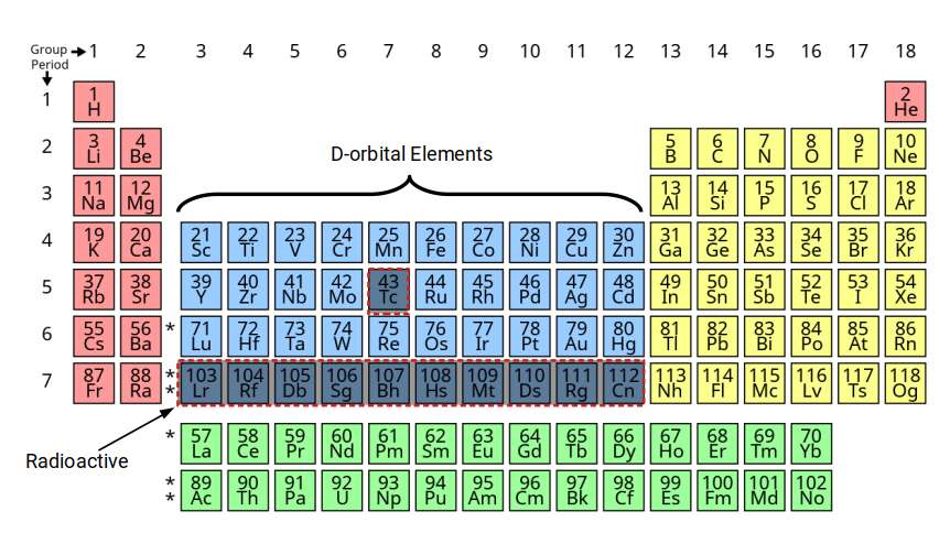
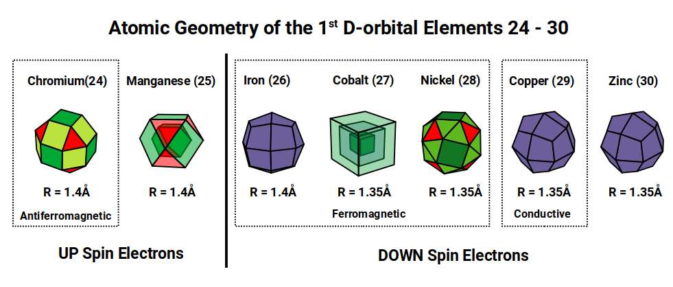
Of the 81 stable elements, only three are ferromagnetic at room temperature. All three appear in the first D-orbital set: Iron (26), which exhibits by far the strongest ferromagnetism, followed by Cobalt (27) and Nickel (28). Antiferromagnetism — the tendency to resist alignment in a magnetic field by adopting alternating spin orientations — is most pronounced in the two preceding elements, Chromium (24) and Manganese (25). In principle, these atoms should be ferromagnetic, since they possess many unpaired D-orbital electrons. Yet compounds of these solids align in opposing directions, cancelling their magnetic properties.
The electron configuration of these elements reveals a clear pattern. Electrons exhibit either an up or down quantum spin value. Both antiferromagnetic elements, Chromium and Manganese, possess a full complement of up-spin D-orbital electrons. Once the up-spin set is complete, the down-spin electrons begin to fill the orbitals. The three ferromagnetic elements — Iron, Cobalt, Nickel — each possess a mixture of filled and half-filled D-orbitals. The next elements, Copper (29) and Zinc (30), have a full complement of D-orbital electrons, just as Chromium and Manganese have a full set of half-filled ones. This is the Aufbau Anomaly, which remains without a satisfactory explanation in conventional chemistry.
Copper (29) and Zinc (30) are not ferromagnetic. However, Copper is one of the best conductors of electricity — only Silver (47) exceeds it marginally. Both are the second-to-last element in their respective D-orbital sets, placing them in group 11. Gold (79) occupies the equivalent position in the third D-orbital set and is the third most conductive element.
One further anomaly deserves attention. With the exception of the first element in the first D-orbital set, all D-orbital elements exhibit an atomic radius of either 1.4 Å or 1.35 Å. Standard theory attributes this uniformity to electron shielding by the D-orbitals — a claim presented without any mathematical derivation. According to the conventional model, increasing numbers of protons and neutrons should progressively reduce the atomic radius. This is simply not observed. Similar uniform radii appear within the P-orbital elements, and current theory offers no explanation.
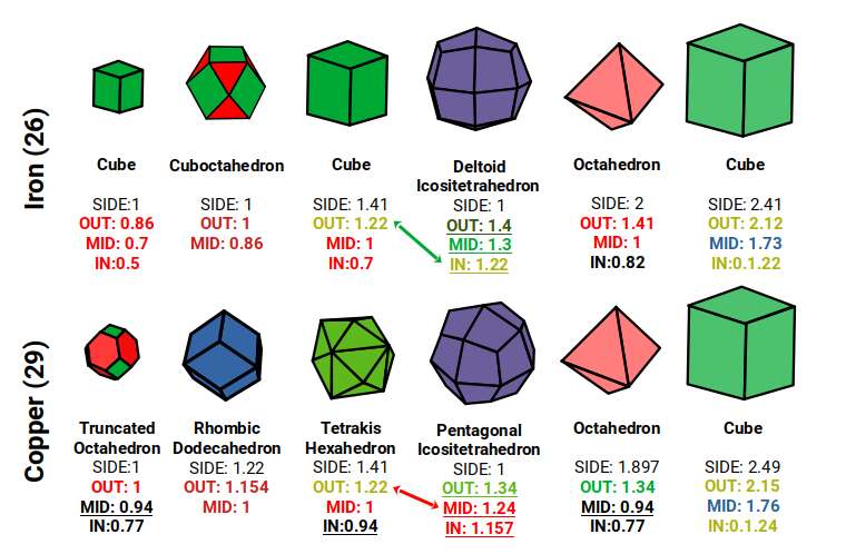
Atomic Geometry provides the answer. The two radii, 1.4 Å and 1.35 Å, arise from the out-spheres of the Rhombic Cuboctahedron, Snub Cube, and their duals. As proton and neutron counts increase, the atom evolves through a sequence of geometric forms. Chromium (24) has 24 protons, matching the corners of the Rhombic Cuboctahedron. Manganese has 55 nucleons, which produces a large Cuboctahedron. Iron's 26 protons match the Dual of the Rhombic Cuboctahedron — the Deltoid Icositetrahedron — at which point the radius falls from 1.4 Å to 1.35 Å for Cobalt, whose 27 protons form a Cube. This collapses the electron cloud geometry into the Snub Cube, which then transitions into its own dual, the Pentagonal Icositetrahedron, for Copper and Zinc.
Atomic Geometry offers a geometric framework that predicts atomic radii more closely than the Bohr model, accounts for the Aufbau anomalies, and provides explanations for the distinct properties of different element types. The remainder of this article builds on this model to examine the geometric basis of magnetic and conductive behaviour. Readers seeking greater depth on the D-orbital geometries themselves will find detailed treatments in the D-orbital geometry series.
Magnetic Orders
Every electron behaves like a tiny bar magnet, with a property called quantum spin — a fixed orientation that can point either "up" or "down". In most materials these spins point in random directions and cancel each other out. In ferromagnetic materials, vast numbers of them align in the same direction, producing a net magnetic field strong enough to pick up a paperclip. Materials can also be antiferromagnetic, where neighbouring spins are forced to alternate, cancelling any net field, or paramagnetic (weakly attracted to magnets) and diamagnetic (weakly repelled). Understanding what determines which category an element falls into is the central problem this article addresses.
Permanent magnets are a commonplace feature of modern technology — from refrigerator magnets to hard disk storage to the generation of electricity. Their existence depends on a property of certain solids in which the quantum spins of large numbers of adjacent atoms align in the same direction.
Iron (26) is the most recognisable magnetic substance on the periodic table. When Iron atoms are arranged in a solid lattice, their electron spins tend to align in the same direction. When an external magnetic field is applied, this alignment is strengthened. In compounds containing more than one element type, ferromagnetic behaviour can persist as long as all atomic spins continue to point in the same direction, regardless of differences in field strength between atoms.
Antiferromagnetic materials behave in precisely the opposite way: electron spins in adjacent atoms alternate in direction, so that any externally applied field causes more atoms to align in opposing polarities rather than fewer. Chromium (24) is the most prominent example.
A third configuration arises when atoms neither align consistently nor alternate regularly. This is called a spin glass, and is often produced by mixing ferromagnetic and antiferromagnetic elements in proportions that create small domains of partial alignment in both orientations.
Temperature plays an important role in all of this. Below a material's Curie Temperature (the threshold beyond which thermal energy disrupts spin alignment — 770 °C for iron), magnetic orientations remain fixed. Above it, atomic spins become free and can be reoriented. This is why a substance can be permanently magnetised by heating it above its Curie Temperature, applying a strong field, and then cooling it.
Materials that are neither ferromagnetic nor antiferromagnetic fall into two further categories. If any orbitals are unpaired — occupied by only one electron — the substance is paramagnetic and will be weakly attracted in a magnetic field. If all orbitals are completely filled, as in Copper (29) or Zinc (30), the substance is diamagnetic and is weakly repelled.
Antiferromagnetic Materials
The most commonly recognised antiferromagnetic element is Chromium (24), followed by Manganese (25). According to conventional theory, elements with unpaired electrons should be ferromagnetic — yet both of these atoms have a full complement of half-filled D-orbitals. When compared to Iron, the most ferromagnetic element, all three exhibit the same radius (1.4 Å) and even form the same body-centred lattice in a compound. Chromium has the same number of neutrons (30) as Iron. Why should these elements exhibit exactly the opposite magnetic behaviour?
Conventional theory offers the explanation that atoms settle into the most energetically convenient configuration — an answer that lacks any geometric or structural content. Atomic Geometry provides a more precise account.
The 24 protons of Chromium define the geometry of the Rhombic Cuboctahedron. This shape can combine with a Cube and Tetrahedron to form a cubic lattice structure. Manganese, with its Cuboctahedral form, can also lattice with Octahedra.
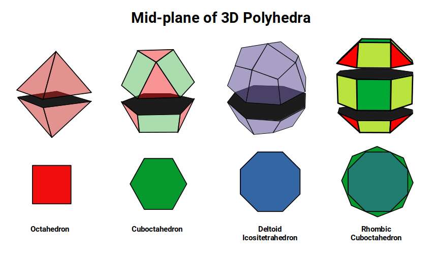
Electrons can only exhibit two quantum states: up or down spin. In the 4D interpretation of the electron field, quantum spin is ascribed to the rotation of a 4D object on its w-axis, which in turn produces quantised rotational steps of the solid around a central axis. In the case of the Rhombic Cuboctahedron and the Cuboctahedron, this midsection is formed by an octagon and a hexagonal plane respectively. As one atom rotates clockwise, adjacent atoms rotate anticlockwise — the same mechanics as a set of interlocking cogs.

The key difference between the cog model and the 4D interpretation is that as a 4D object rotates on its w-axis, it momentarily ceases to exist in 3D space. Only as it completes a full rotation does it re-enter the third dimension, producing discrete frames of interaction. This rotational speed is governed by the speed of light, which unifies the 4D rotation throughout the material and produces the quantised effects of electron spin. This view represents a significant departure from the continuous model of time implied by conventional spacetime, and provides a geometric explanation for the quantised nature of the electron cloud — including the otherwise unexplained phenomenon of electrons jumping between shells.
When Chromium is mixed with an impurity such as oxygen, its antiferromagnetic properties give way to ferromagnetism. In geometric terms, the impurity atoms act as counter-rotating elements within the lattice, realigning the Chromium atoms so that all spins point in the same direction. A similar mechanism applies to Manganese, whose magnetic properties are transformed by the addition of other elements that increase the inter-atomic spacing.
The Deltoid Icositetrahedron and Ferromagnetism
Iron (26) is the most ferromagnetic element on the periodic table. Conventional theory attributes this to its many unpaired electrons — yet this is equally true of Ruthenium (44) and Osmium (76), both of which have an identical number of unpaired D-orbital electrons and display no ferromagnetic behaviour whatsoever. Unpaired electrons are therefore not a sufficient explanation.
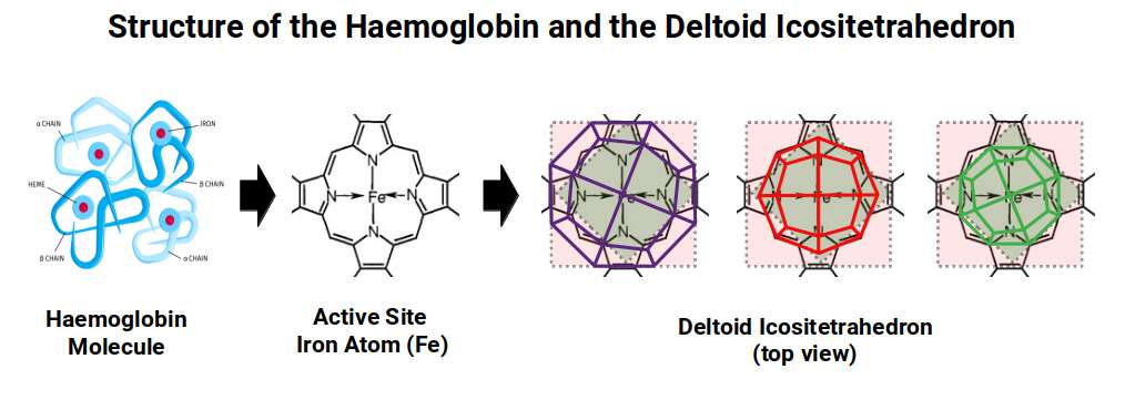
Atomic Geometry ascribes the 26 protons of Iron to the Deltoid Icositetrahedron — a 24-faced solid whose faces are all identical kite shapes, and which is the geometric dual (mirror-complement) of the Rhombic Cuboctahedron. While the Rhombic Cuboctahedron is composed of two types of face — squares and triangles — the Deltoid Icositetrahedron is composed of a single type: the kite face.
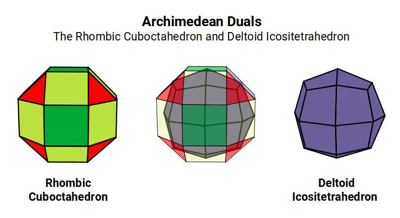
The construction of these duals can be understood from the relationship between a Cube and an Octahedron. In the Rhombic Cuboctahedral model, a Cube with side length √2 nests inside the solid with its corners centred on each triangular face. An Octahedron places its corners at the centre of the square faces on the x, y, and z axes. As the Deltoid Icositetrahedron forms by swapping places with its dual, these corners push through the centre of each face. The Octahedron grows to match the out-sphere of the Iron atom, while the Cube reduces slightly, bringing both into a unified compound. This is most clearly seen in a 2D projection.
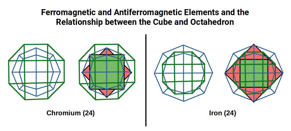
This gives rise to the Rhombic Dodecahedron, which is the template for the 4D hypercube — and, as we shall see shortly, the Brillouin zone of the body-centred cubic lattice of Iron.
The second geometric reason for Iron's exceptional ferromagnetism lies in the nature of rotation. Within the D-orbital set, one of the five orbitals takes a toroidal form with two lobes oriented north-south. The Rhombic Cuboctahedron is the only Archimedean Solid that exhibits an octagonal midsection capable of being rotated, matching the toroidal orbital geometry. When the Deltoid Icositetrahedron forms, this midsection flattens into a single plane, allowing the solid to be rotated in two independent halves. The octagonal shape is preserved but rotated 22.5° relative to the original.
In the Rhombic Cuboctahedral lattice, flat faces of adjacent atoms touch each other so that as one atom rotates clockwise its neighbour rotates anticlockwise — producing antiferromagnetism. In the Deltoid Icositetrahedral lattice, it is the corner points of the octagonal midsection that meet, not the flat faces. This spacing means that adjacent atoms are no longer constrained to rotate in opposite directions: they can rotate together, unifying their spin orientation and producing the ferromagnetic properties of the Iron lattice.
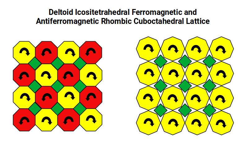
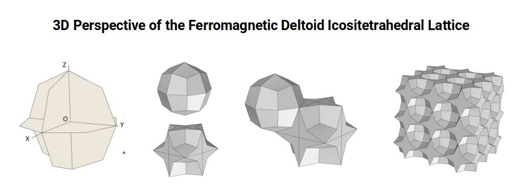
Furthermore, the Deltoid Icositetrahedron exhibits a single mid-plane in the vertical direction, allowing a similar rotational coupling between the layers above and below. When assembled into a cubic arrangement, each atom is spaced apart by a four-pointed star, which extends unified spin alignment over a much wider volume.
An intriguing biological parallel appears here. Iron plays a central role in haemoglobin, the molecule that binds oxygen in red blood cells. The active site contains four nitrogen atoms arranged in a square, with a single Iron atom suspended at the centre. The projection of the Deltoid Icositetrahedron can be superimposed over this active site at various scales and orientations. Furthermore, Nitrogen has 7 protons and 7 neutrons; four nitrogen atoms therefore total 56 nucleons — the same count as the Iron atom itself. This geometric correspondence between the carrier atom and its binding architecture has not been recognised in conventional biology, and opens a new avenue for understanding this mechanism essential to all red-blooded life.
As noted above, Chromium (24) has 24 protons matching the corners of the Rhombic Cuboctahedron, and Manganese (25) has 55 nucleons fitting the Cuboctahedral form. Iron, at 26, marks the last element at 1.4 Å before the atomic radius drops to 1.35 Å as the D-orbital structure collapses into the Snub Cube.
Snub Cube Magnetic Order
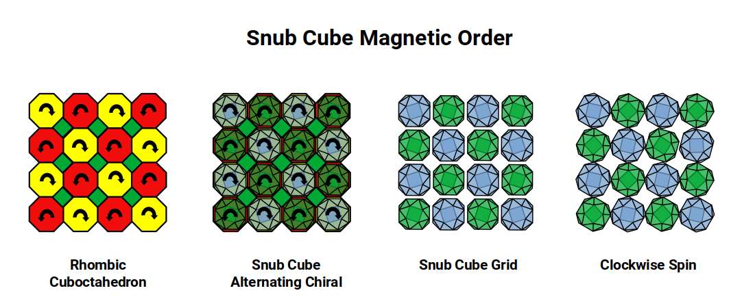
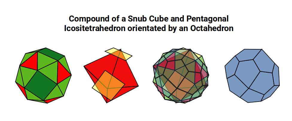
After Iron (26), all remaining D-orbital elements in the first set share the same atomic radius of 1.35 Å. This shift corresponds geometrically to the collapse of the Rhombic Cuboctahedron into the Snub Cube — a transformation known as the Extended Jitterbug. Like the Rhombic Cuboctahedron, the Snub Cube has 24 corners. The key difference is that the diagonal across 12 of the Rhombic Cuboctahedron's square faces collapses into two triangles. This is achieved by a 22.5° rotation of the faces on the x, y, and z axes, reducing the out-sphere from 1.4 Å to 1.35 Å — precisely the step between Iron and its successors.
The Snub Cube is a chiral geometry: its square faces can be rotated either clockwise or anticlockwise, producing two mirror-image versions of the same form. When placed in a lattice, a clockwise version will induce anticlockwise rotation in its immediate neighbours — the same cog-like effect seen in the Rhombic Cuboctahedral lattice. However, as each solid contracts in size, gaps open between adjacent atoms. Within those gaps, adjacent atoms are free to rotate in the same direction, allowing spin alignment and producing ferromagnetism.
After Iron, the only other elements that are ferromagnetic at room temperature are Cobalt (27) and Nickel (28), to a considerably lesser degree. In Atomic Geometry, Cobalt's 27 protons form a cubic arrangement as the geometry transitions toward the Snub Cube for Nickel (28).
The Snub Cube offers a wide variety of possible lattice configurations. When placed corner-to-corner, the shape of the inter-atomic space resembles the Deltoid Icositetrahedral lattice but with two different side lengths. When viewed in 2D projection these alternate on the x and y axes. The form can also be oriented to produce a rhombic spacing or an offset star, depending on chirality. When flat faces are placed against each other, two further orientations emerge depending on whether square or triangular faces make contact.

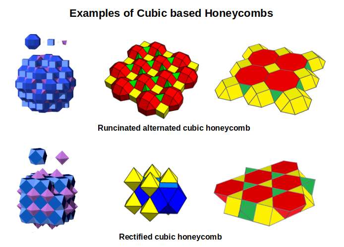
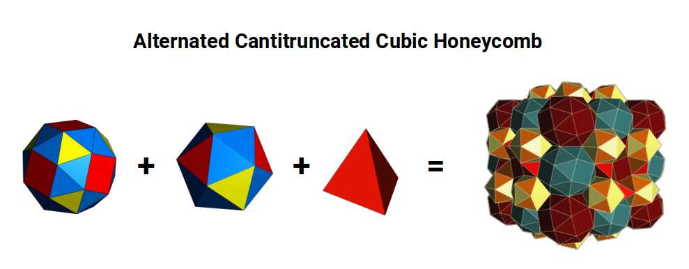
In three dimensions, the only recognised space-filling structure that includes the Snub Cube is the Alternated Cantitruncated Cubic Honeycomb, which contains Snub Cubes in alternating chiral symmetries. The gaps between them are filled with Tetrahedra and Icosahedra exhibiting two side lengths in the ratio 1:1.04277 — making it a near-miss regular polyhedral structure.
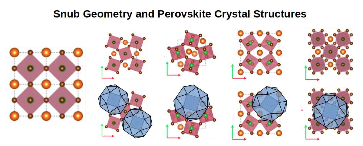
The Snub Cube does not currently appear in the literature of mainstream chemistry. However, a class of lattice called Perovskite crystals exhibits a closely related rotational phenomenon. Perovskites are formed from octahedral configurations of smaller atoms interspersed with larger-radius atoms, and just like the square faces of the Snub Cube, these octahedra can be rotated to produce a wide variety of lattice types. The result is a class of adaptive materials capable of exhibiting colossal magnetoresistance, ferroelectricity, superconductivity, and charge ordering — even when the individual component elements display none of these properties in isolation. These materials have broad applications in electrical sensors, high-temperature superconductors, and fuel cells.
The reason the snubification of these elements is not recognised in the literature appears to be that chemistry tends to observe crystal structures rather than the invisible geometry that allows those structures to be manipulated. Atomic Geometry proposes that it is the Snub Cube operating within the crystal lattice that produces the rotational behaviour responsible for these exotic properties.
Magnetic Domains and the Tribonacci Constant
A bar magnet is not uniformly magnetised at the atomic level. It is divided into magnetic domains — regions, each containing billions of atoms, within which all spins point the same way. Neighbouring domains may point in different directions. When the domains are randomly oriented, the material has no net magnetism. When they align — pushed by an external magnetic field, or locked in during cooling — the material becomes magnetised. This is why you can demagnetise a magnet by dropping it: the shock scrambles the domains. The question of what determines the size and geometry of these domains has not been resolved by conventional physics. Atomic Geometry offers a proposal.
The capacity of a material to display magnetic properties depends on the alignment of quantum spins across large groups of atoms — the so-called magnetic domains. A magnetic material contains multiple domains in which atoms are locally aligned. When an external field is applied, some domains grow at the expense of others and shift toward alignment with the field. If one domain is larger, it will tend to influence smaller ones. If domains are equal in size, their effects cancel — which is why even Iron, the most ferromagnetic material, can be demagnetised.
Conventional domain theory provides a surface-level account but cannot explain what determines the size and geometry of domains in the first place, nor why domains re-establish themselves reproducibly when a material is cooled after being heated above its Curie Temperature. Atomic Geometry offers a structural explanation, and it depends on a property unique to the Snub Cube.
The Snub Cube is the only Archimedean Solid that encodes the Tribonacci constant within its geometry. The Tribonacci numbers are generated by adding together the three preceding terms of a series, starting with 0, 0, 1:
Fibonacci Numbers: 1, 1, 2, 3, 5, 8, 13, 21, 34, 55, 89, 144…
Tribonacci Numbers: 0, 1, 1, 2, 4, 7, 13, 24, 44, 81, 149, 274…
Both series contain the number 13, which corresponds to the Cuboctahedron and is half the proton count of Iron. The Tribonacci series then produces 24 — the number of corners of the Rhombic Cuboctahedron — followed by 44 and 81. Notably, element 43 is anomalously radioactive among the otherwise stable elements, after which element 44 begins a new block of stable elements. This gives a total of exactly 81 stable elements — both values appearing sequentially in the Tribonacci series.
Just as the Golden Ratio is approximated by dividing adjacent Fibonacci numbers, the Tribonacci constant (η ≈ 1.839) is approximated by dividing adjacent Tribonacci numbers (for example, 24 ÷ 13, or 81 ÷ 44). The defining algebraic property of the Tribonacci constant is the cubic analogue of the Golden Ratio's quadratic identity:
The Golden Ratio: Φ² – Φ – 1 = 0
The Tribonacci Constant: η³ – η² – η – 1 = 0
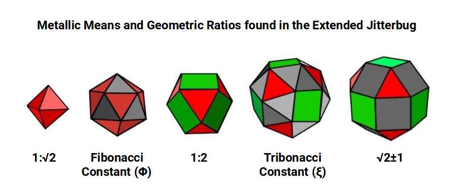
Within the Extended Jitterbug sequence, each geometric form expresses a characteristic mathematical ratio. The Cuboctahedron expresses the ratio 1:2. The Rhombic Cuboctahedron expresses the Silver Ratio (√2 ± 1) through its octagonal midsection. The Icosahedron expresses the Golden Ratio through its pentagonal structure. The Snub Cube stands apart: in losing its midsection through the 22.5° rotation, it gains the Tribonacci constant instead.
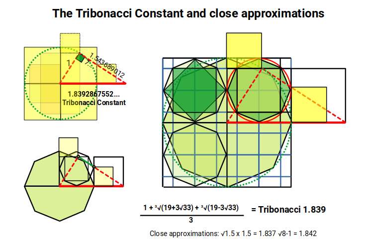
The Tribonacci constant (η ≈ 1.839) can be geometrically constructed from a circle of radius 1 placed inside a square. When a right-angled triangle is rotated away from the vertical until the distance from its right angle to the vertical equals the distance from the right angle to the horizontal, the resulting hypotenuse equals the Tribonacci constant. A close approximation is given by √8 − 1 and by √1.5 × 1.5.
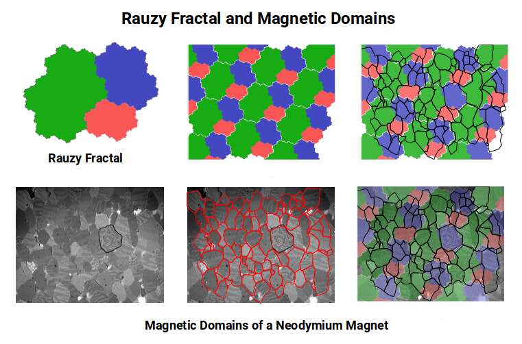
The Tribonacci constant also generates a Rauzy fractal — a shape that tiles a flat surface in three sizes that are exact replicas of one another, each proportional to the others in a ratio satisfying the Tribonacci series. The tessellation of the Rauzy fractal bears a remarkable resemblance to the formation of magnetic domains in a ferromagnetic material. When the Rauzy fractal is superimposed over a cross-section of such a material, large regions of coherence appear.
This correlation applies directly to Cobalt (27) and Nickel (28), which share the Snub Cube geometry and the Tribonacci constant encoded within it. But what about Iron, which is assigned the Deltoid Icositetrahedron at a radius of 1.4 Å and appears to have no direct connection to the Tribonacci constant?
Here, a new geometric relationship emerges. In Atomic Geometry, the radius of 1.4 Å arises from a Rhombic Cuboctahedron with a side of 1. When this transforms into its dual, two distinct edge lengths appear: the longer edge (A) = 1.1589 and the shorter edge (B) = 0.8964. Their ratio is given by:
A × (4 + √2) / 7
When scaled to the values of the Deltoid Icositetrahedron in the Atomic Geometry model, this ratio is extremely close to the Tribonacci constant divided by √2:
(A ÷ B) ≈ (η ÷ √2)
The exact value of this ratio is √8 − 1 — which, as noted above, is the close geometric approximation to the Tribonacci constant. Since 1:√2 is the ratio of a square's side to its diagonal, the Tribonacci constant is expressed in the diagonal of the Iron lattice when viewed in 2D projection. This diagonal relationship is what produces the large magnetic domains unique to Iron.
This is the first proposal to find an expression for the Tribonacci constant in a physical system, and it opens new lines of investigation into the geometric mechanisms that form magnetic domains.
The Geometric Rules of Paramagnetic and Diamagnetic Elements
While Iron, Cobalt and Nickel are ferromagnetic, the next elements in the first D-orbital set — Copper (29) and Zinc (30) — are not. They are instead diamagnetic: weakly repelled by an applied magnetic field. Conventional theory attributes diamagnetism to the complete filling of all orbital shells with both up and down spin electrons. But closer examination shows this is not a reliable rule. The majority of P-orbital elements are diamagnetic regardless of whether their orbitals are fully filled. Helium has a half-filled S-orbital and is also diamagnetic. The electron-pairing rule, like the ferromagnetic unpaired-electron rule, does not hold up across the full periodic table.
Atomic Geometry provides a more consistent account. P-orbitals are assigned the geometry of the Octahedron; D and F-orbitals are assigned the geometries of the Cube and Cuboctahedron respectively. As a general rule: elements with Octahedral geometry (P-orbital elements) are diamagnetic, while elements with Cubic or Cuboctahedral geometry (D-orbital elements) tend to be paramagnetic or ferromagnetic. The exceptions among D-orbital elements are those with fully paired electrons. Apparent exceptions elsewhere — such as oxygen (8), whose 16 neutrons produce a hypercubic configuration, and aluminium (13), whose 13 protons define a Cuboctahedron — can be explained by the specific geometric forms that their nucleon counts impose.
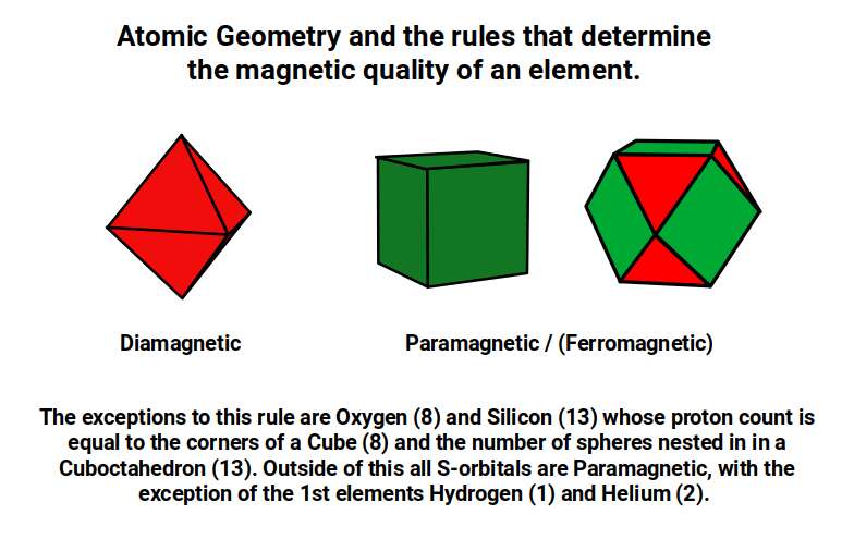
Atomic Geometry therefore not only provides a geometric explanation for the ferromagnetic qualities of Iron, Cobalt and Nickel — it also offers a far more accurate framework for predicting the paramagnetic and diamagnetic properties of all 81 stable elements, including those that apparently contradict standard rules.
Bloch's Theorem vs the Drude Model
Before examining Copper's conductivity in geometric terms, it is worth clearing up a widespread misconception about what electricity actually is at the atomic level. Most of us were taught something like the "Drude model" — electrons as tiny charged balls rolling along a wire like marbles through a pipe. This picture is wrong, and has been known to be wrong for over a century. The correct picture, established by Felix Bloch in 1928, is that electrons in a crystal are not particles at all in the classical sense: they are waves spread across the entire lattice. Bloch's Theorem (the mathematical statement of this) is the foundation of all modern semiconductor physics. Without it, transistors, LEDs and microchips could not be designed. Keeping this wave picture in mind is essential for understanding the geometric argument that follows.
The exceptional conductivity of Copper is commonly taught as a consequence of its having a full set of paired D-orbital electrons and only one S-orbital electron in its outer valence shell. The idea is that the D-orbitals bond with each other, leaving the single outer electron free to travel through the material. However, like many superficial accounts in mainstream physics, this model does not survive scrutiny. Chromium (24) also has only a single electron in its outer shell, yet exhibits no particular conductivity. Several elements in the second D-orbital set — elements 41, 42, 44 and 45 — also carry a single outer S-orbital electron without any exceptional conductivity.
One might argue that conductivity requires both fully paired D-orbitals and a single outer S-orbital. Gold and Silver fit this description and are indeed highly conductive. But the fourth most conductive element is Aluminium (13), which is not a D-orbital element at all and has three valence electrons in its outer shell. And Cobalt (27), which is ferromagnetic, is more conductive than Zinc (30). Clearly, the number of paired electrons and the configuration of the outer shell are not the determining factors.
The deeper problem is the persistence of the particle model of the electron. It has been demonstrated experimentally that electricity does not flow through a wire in the way commonly imagined. It is the magnetic field that establishes the electric field. Electricity can be transmitted wirelessly and can reach an adjacent bulb before the current has traversed the wire. The wire guides the circuit and generates a secondary magnetic field stronger than the primary — but the energy transport is fundamentally electromagnetic, not a flow of particles. In 4D Aether theory, there is no particle: only an electron wave. The wave-only model is not recognised in conventional physics because the particle model of light was established at the turn of the twentieth century as the solution to the photoelectric effect and ultraviolet catastrophe. However, investigation of the mathematics behind those experiments reveals a flaw in that reasoning — examined in detail in the 4D Aether articles.
The Drude model of electrical conduction is still routinely taught today solely for its simplicity, despite having been disproven. The correct picture requires treating electrons as waves. This is not a theoretical abstraction: it is the physical reality on which modern computing depends. Transistors do not work by producing holes in doped material — they work through quantum tunnelling, which appears mysterious and paradoxical only when viewed from the particle perspective. Viewed as an evanescent wave phenomenon penetrating a material through wave coupling, the mechanism is straightforward. Concepts such as the drift velocity of electrons are purely theoretical: no one has ever measured an electron in motion, and no one has ever established a definite electron radius. The only model consistent with the full range of observed electromagnetic phenomena is the wave model — and once the 4D Aether is reintroduced, removing the need for the photon as a particle, the quantum enigmas that plague the standard model resolve into coherent geometry.
Electron Waves and the Tribonacci Constant
Having established the wave character of the electron and the inadequacy of the particle model for explaining conductivity, we can now examine why Copper has the conductive properties it does.
After Nickel (28), the next element, Copper (29), acquires a full set of paired D-orbital electrons. Alongside the transition from ferromagnetic to diamagnetic behaviour, Copper gains an exceptionally high conductivity. In Atomic Geometry, Copper is assigned the Pentagonal Icositetrahedron — the dual of the Snub Cube. This is the same structural relationship that exists between Chromium (antiferromagnetic, Rhombic Cuboctahedron) and Iron (ferromagnetic, Deltoid Icositetrahedron). In each case, the transition from a form to its dual produces a dramatic change in physical properties.
The Pentagonal Icositetrahedron exhibits 38 corners. This is the precise midpoint between the atomic number of Copper (29) and Silver (47): 38 − 9 = 29 and 38 + 9 = 47. Although Silver is marginally more conductive than Copper (0.63 × 10⁶/cm Ω vs. 0.596 × 10⁶/cm Ω), both elements occupy the second-to-last position in their respective D-orbital sets — and both share the same geometric form.
Like the Snub Cube, the Pentagonal Icositetrahedron encodes the Tribonacci constant in the ratio of its two edge lengths. The exact formula is a ÷ (s + 1), where a is the longer edge and s = (η − 1) ÷ 2. Dividing the longer edge (a) by the shorter edge (b) produces a result close to √2:
Deltoid Icositetrahedron (Iron): (A ÷ B) ≈ (η ÷ √2)
Pentagonal Icositetrahedron (Copper): (A ÷ B) ≈ √2
The ratio between the geometry of Iron — the most ferromagnetic element — and Copper — the most conductive in the set — differs by a factor of exactly the Tribonacci constant. This reveals a deep geometric relationship: the magnetic field (Iron, Silver Ratio domain) and the electric field (Copper, Golden Ratio domain) are separated by the Tribonacci constant.
Yet in Atomic Geometry, Zinc (30) is assigned the same geometry as Copper. So why is Zinc not equally conductive?
The answer lies in the isotope distribution of each element. Copper (29) is anomalous among D-orbital elements with an odd proton count: it is the only one to exhibit two stable isotopes. Approximately one third of all copper atoms have 36 neutrons; the other two thirds have 34 neutrons. Silver similarly has two isotopes with an odd proton count. D-orbital elements with an even proton count tend to have four stable isotopes, while Zinc (30) has five.
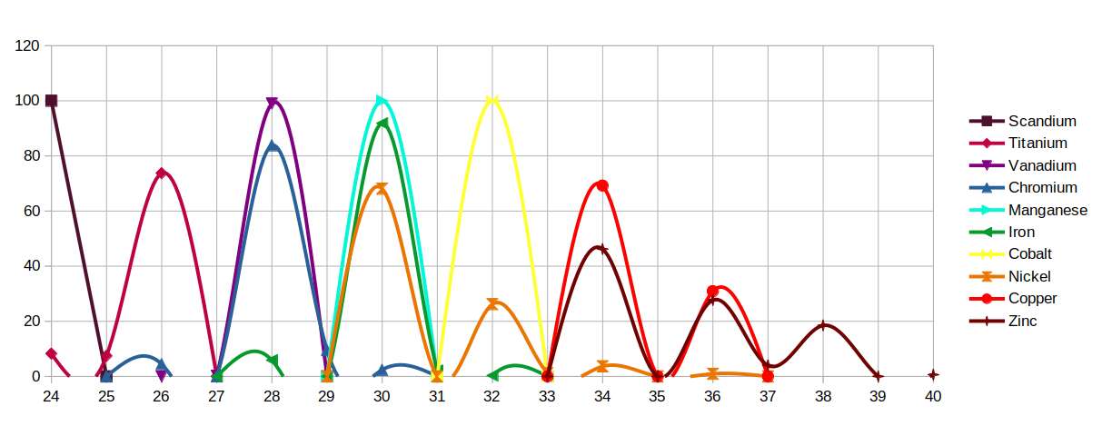
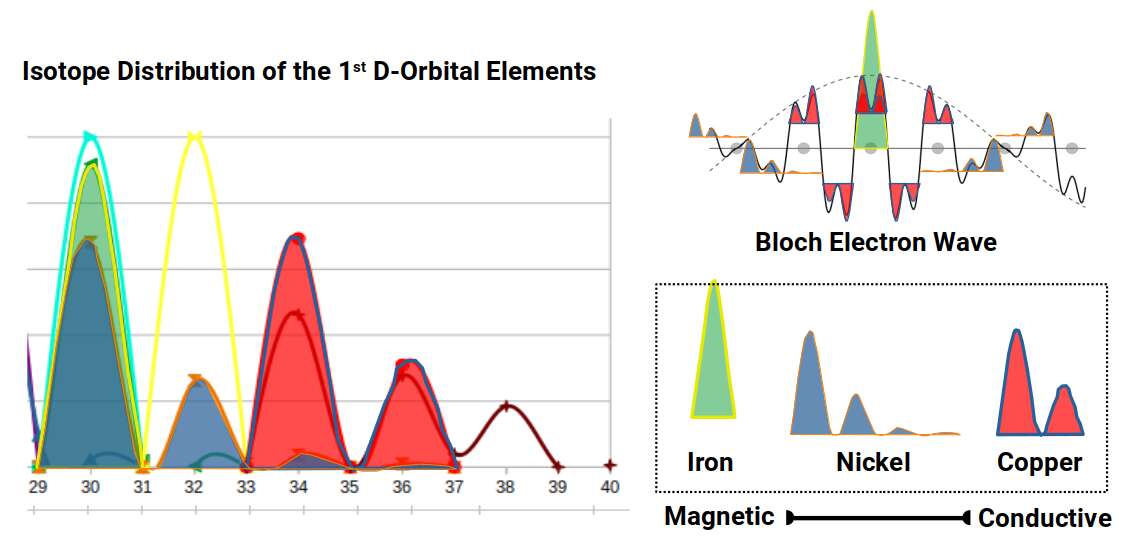
The percentage distribution of isotopes varies considerably. Around 90% of Iron exhibits 30 neutrons, producing an unusually sharp single-peak profile for an even-proton element. Cobalt, with an odd proton count, has only a single isotope. Nickel distributes across several isotopes, with roughly two thirds at 30 neutrons and the remainder spread to 36. Zinc's five isotopes are distributed more evenly: just under half at 34 neutrons, just under a third at 36, then diminishing fractions up to 40 neutrons.
When the isotope distributions are plotted, the peaks for Iron, Cobalt and Nickel align with the peaks of Copper in a precise geometric pattern — two parallel lines connecting the magnetic elements to the conductive one.
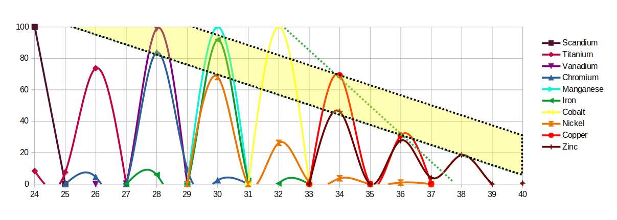
Extracting the profiles of Iron and Copper, their combined waveform — Iron's single dominant peak truncated by Copper's double peak — closely resembles the Bloch electron waves that describe the propagation of electricity through a lattice. Similar waveforms can be constructed by substituting Cobalt or Nickel for Iron.
This correlation does not constitute a proof, and the exact frequency ratios governing the Bloch electron wave are not yet fully established. However, there is a further clue in the nature of N-bonacci numbers — the family of series of which the Fibonacci and Tribonacci are members.
For any N-bonacci series — Fibonacci (2 terms), Tribonacci (3 terms), four-bonacci (4 terms), and so on — the ratio of adjacent terms converges to a unique constant regardless of the starting values chosen. Remarkably, as the number of terms approaches infinity, this constant approaches 2. Every calculation that can be performed reduces to two numbers acted upon by an operator producing a third — which means every calculation is, in some sense, Tribonacci in nature.

A further dimension opens when the additive rule is replaced by subtraction. For Fibonacci subtraction, starting with 1 and 1, the series becomes 0, 1, −1, 2, −3, 5, −8, 13, −21 — alternating positive and negative Fibonacci numbers — and when adjacent terms are divided, the result converges to −Φ. Extending this to three terms (Tribonacci subtraction), rather than converging to −η, the series generates an erratic, wave-like set of numbers that shifts dramatically with even tiny changes in the starting values.
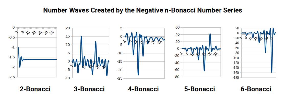
The connection to quantum mechanics is this: the Schrödinger equations that underpin all of quantum theory are, at their core, descriptions of waveforms evolving in 3D space. They are so computationally demanding that even the helium atom — two electrons — cannot be modelled accurately. The negative N-bonacci calculator offers a potential alternative: by inputting just three numbers it generates a waveform. By the six-bonacci level, the emerging waveform begins to resemble the periodic electron waves predicted by Bloch's theorem. Inputting the atomic numbers 29 (Copper) : 26 (Iron) : 3 (their difference) generates a waveform that resembles the transport mechanism of a conductive electron wave.
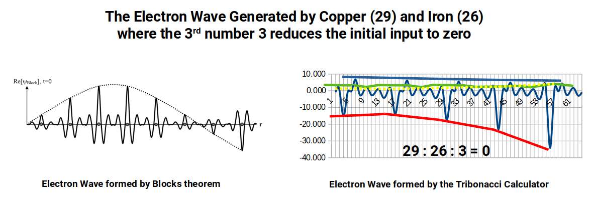
This approach derives from 4D Mathematics — a theoretical framework that we developed from early 2022. There is significant uncharted territory to explore, and the correlations presented here are preliminary. They do, however, suggest a simpler alternative to the Schrödinger approach for modelling electromagnetic waves in lattices.
Golden and Silver Ratios in Magnetic and Conductive Elements
With the wave character of both the magnetic and conductive fields established in terms of geometry, we can examine the precise numerical values of those fields across the first D-orbital set and discover that the fundamental geometric ratios — the Silver Ratio, the Golden Ratio and the Tribonacci constant — appear directly in the measured physical quantities.
The ferromagnetic strength of Iron, Cobalt and Nickel, measured in emu per cm³, mirrors a sequence of geometric ratios. Iron's field strength is approximately √3, or more precisely √0.5 + 1 — which can also be expressed as the Silver Ratio with the +1 replaced by +2, divided by 2. Cobalt's field strength is approximately √2. Nickel's is approximately √2 ÷ 3. The difference between Iron and Nickel is ((√2 + 1) × 3) ÷ 3. The Silver Ratio is thus expressed through the magnetic properties of the three ferromagnetic elements.
The conductive properties of the same elements, measured in cm Ω and scaled to the appropriate magnitude, show the ratios of the in-sphere, mid-sphere, and out-sphere of a Cube: Iron ≈ 1, Nickel ≈ √2, Cobalt ≈ √3.
For the conductive elements, Copper and Silver both have conductivities that approximate 1/Φ (= 0.618) at this scale — equivalently, the ratio 5√5 − 5. The Golden Ratio, constructed from √5, governs the electric field just as the Silver Ratio, built from √2, governs the magnetic field. Zinc (30), immediately after Copper, has a conductivity close to Φ itself. Gold (79), the third most conductive element, has a conductivity of approximately Φ² × √3.
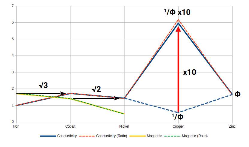
Cobalt (27) is a particularly instructive case. Its 27 protons (= 3³) form a Cube; its 32 neutrons match the corners of a 5D Cube (Rhombic Triacontahedron). The ratio between its magnetic and conductive properties is √2 : √3 — the ratio between the mid-sphere and out-sphere of a Cube. And it is more conductive than Zinc (30), so the sequence of conductivity in the set descends from √3 (Cobalt), through Φ (Zinc), to √2 (Nickel).
When both datasets are combined, the full picture becomes visible. Beginning at Iron (magnetic strength ≈ √3), ferromagnetism drops across Cobalt to Nickel as conductivity rises from 1 to √3 in Cobalt and then falls back to √2 in Nickel. At Copper (29), ferromagnetism vanishes entirely while conductivity leaps to 1/Φ — amplified by a factor of 10. This leap is the geometric fingerprint of the transition from magnetic to electric dominance, mediated by the Phi ratio. After Copper, Zinc's conductivity falls to Φ.
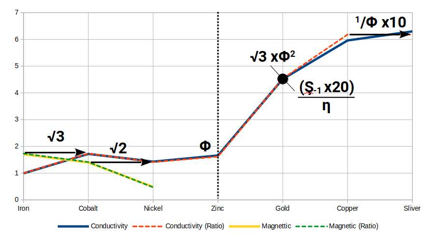
Silver (47) occupies the same position in the second D-orbital set as Copper does in the first. It exhibits an unusually large radius — equal to Φ — and a conductivity just above that of Copper. Gold (79), in the equivalent position in the third D-orbital set, has a conductivity close to (√2 − 1) × 20 ÷ η, where η is the Tribonacci constant. In Gold, the Golden Ratio, the Silver Ratio, √3 and the Tribonacci constant converge in a single expression — a remarkable geometric unity.
Brillouin Zones and the Geometry of Electron Waves
Imagine the crystal lattice as a series of radio transmitter towers arranged in a perfect grid. When you send a wave signal across this grid, some frequencies travel freely, some bounce back, and some are blocked entirely — depending on the spacing between towers. Physicists map these allowed and forbidden frequencies into a mathematical space called reciprocal space (or k-space), where the geometry of the crystal is represented in terms of its wave-propagation properties rather than its physical positions. The boundaries of the allowed regions in this map are the Brillouin zones — named after the French physicist Léon Brillouin who formalised the theory in 1930.
The magnetic and conductive properties of elements emerge not just from individual atomic geometries but from how those geometries propagate through the lattice as waves. To analyse this, physicists use the concept of reciprocal space, or k-space: a mathematical representation of the lattice structure that maps the allowed and forbidden regions for wave propagation. The boundaries of these regions are the Brillouin zones.
Many D-orbital lattices are organised into either a body-centred cubic (BCC) or a face-centred cubic (FCC) configuration. When viewed face-on, these form square arrangements representable on a 2D grid.
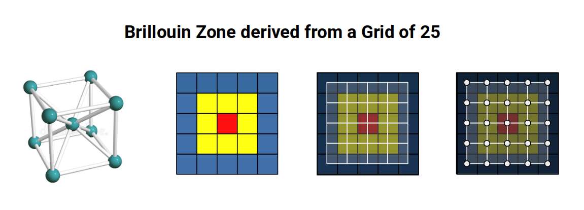
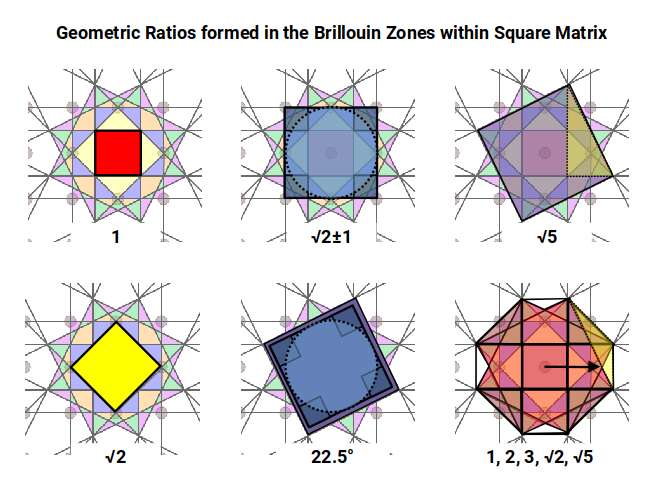
This framework — Brillouin zones — is used to predict many of the properties of elements and compounds in the solid state. The animation below shows how the first six Brillouin zones are constructed on a square grid.
Examining the geometry of these zones reveals a precise sequence of ratios. The first zone (red) is a square with side 1. The second (yellow) is a larger square rotated 45°, with side √2 — the Silver Ratio. The third (blue) forms a cross with its corners removed: those four missing corners, combined, have the same area as the inner unit square, again expressing the Silver Ratio. The fourth zone (orange) introduces two squares with side √5, rotated at the same angle as the square faces of the Snub Cube and encoding the Golden Ratio through the 1:2:√5 right-angled triangle. The sixth zone (final image) forms an octagonal shape measuring 3 on each axis with sides of 1 and √2, encoding both the Silver and Golden Ratios simultaneously.
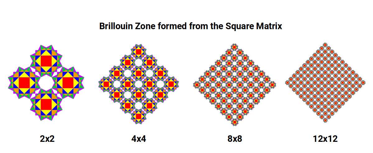
When four Brillouin Zone templates are tiled together, octagonal spaces form at each junction. As the tiling expands, the ratio between zone-occupied area and inter-zone space follows a pattern of successive square numbers — the same mathematical mechanism that governs the expansion of atomic electron shells.
Beyond the square matrix, the only other regular 2D tiling is the hexagonal plane, constructed from equilateral triangles. Its Brillouin zones can be arranged in two orientations; when both are superimposed, the gaps in the circles disappear and the result is the Flower of Life — a motif found throughout sacred geometry, in which the six-pointed star at the centre of each zone is the Star of David.
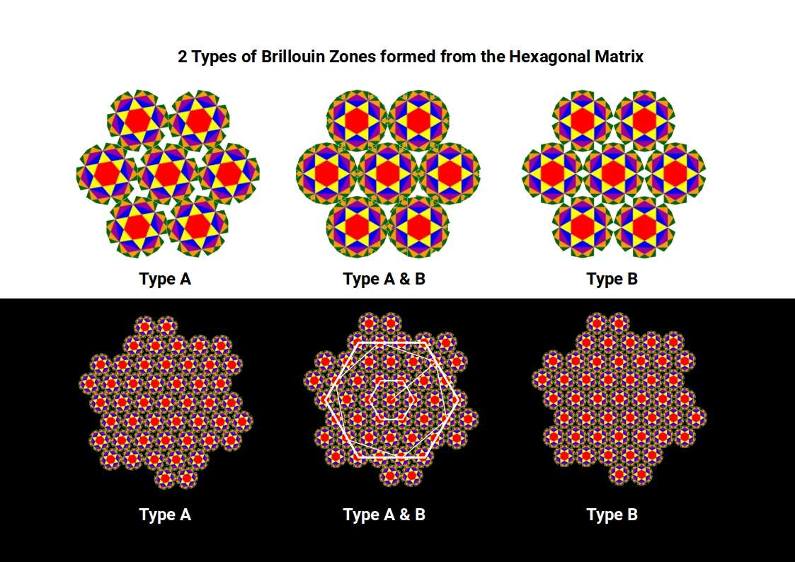
As the hexagonal tapestry expands, successive generations rotate, and the inter-centre spacing becomes √7. This value is close to ³√(3√33), which appears in the exact algebraic formula for the Tribonacci constant — a further thread connecting the geometry of the wave lattice to the constant that governs the conductive and ferromagnetic elements.
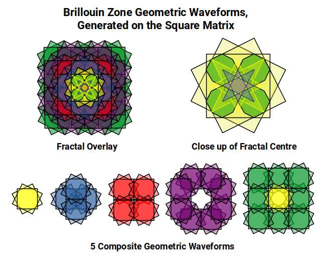
Overlaying Brillouin Zone templates at each adjacent grid point produces a layered fractal that can be grouped into five configuration types. The first is a single cell; subsequent types place zones on the cardinal axes, then the diagonals, creating progressively more complex overlapping patterns. When all five are combined, the central motif is four small octagons — the same construction that provides the geometric approximation of the Tribonacci constant derived earlier from the Silver Ratio fractal. Each octagon is rotated 22.5° within its square frame, exactly the rotation that occurs as the Rhombic Cuboctahedron transforms into the Deltoid Icositetrahedron — the geometry of Iron.
The hexagonal tapestry generates a triangular lattice of overlapping hexagons that can be divided into 12 parts — formed by four triangles at 90° or three squares at 120°.
Brillouin Zones and Atomic Geometry
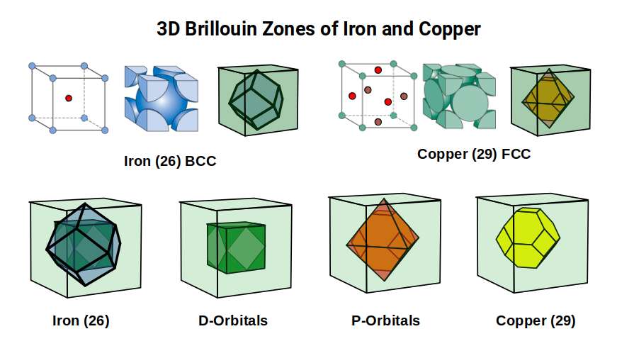
The 2D analysis of Brillouin zones is preparatory groundwork for understanding the 3D structure. Iron forms a body-centred cubic (BCC) lattice — a cube of atoms with one extra atom sitting at the exact centre, like a box with a ball floating in the middle. Copper (29), Silver (47) and Gold (79) all adopt a face-centred cubic (FCC) configuration — a cube with extra atoms at the centre of each face, like a box with a ball pressed against every side wall. These are two of the most common ways atoms pack together in metals, and they produce dramatically different wave-propagation properties. Each lattice type produces a completely different Brillouin zone geometry.
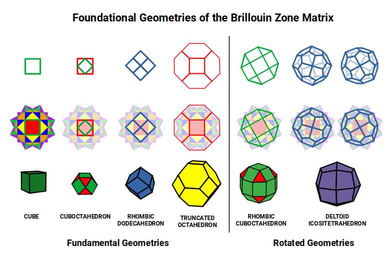
Iron's BCC lattice produces a Brillouin zone shaped as a Rhombic Dodecahedron — the template for the 4D hypercube. The FCC lattice of the conductive elements produces a Truncated Octahedron. In both cases, the corners of the zones are defined by the Octahedron — the geometry of the P-orbitals in Atomic Geometry, while the Cube defines the D-orbital lattice geometry itself.
In 4D geometry, the Rhombic Dodecahedron orients the centres of six surrounding Cubes; together with the enclosing Cube, these create the cubic faces of the 4D solid. Similarly, 12 Rhombic Dodecahedra can be nested inside a Truncated Cuboctahedron.
Within the 2D Brillouin zone representation, a single unit fits exactly inside the projection of a Truncated Octahedron. The projection of the Rhombic Dodecahedron overlays the square units, oriented at 45° to the central square. The 3D geometry of the Brillouin zones is therefore already embedded in the 2D representation.
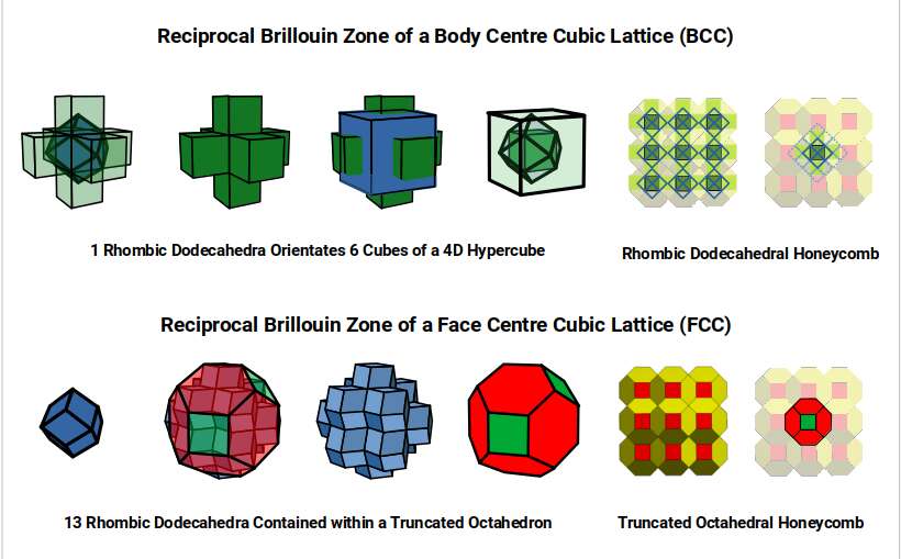
The Brillouin zone tapestry on the square lattice is, in 3D, a Truncated Octahedral honeycomb. Each unit contains a matrix of Rhombic Dodecahedra, spaced one unit apart. At the centre of each unit a Cube is found, truncatable to form a Cuboctahedron (appearing in projection as a square rotated 45°). Over this, the Rhombic Dodecahedron forms as four squares arranged in a larger square — again rotated 45° to the inner Cube.
Each corner of the Rhombic Dodecahedron falls at the halfway point of the four adjacent squares, marking where the cubic faces of the 4D hypercube are located, each shared between adjacent cubes in the grid. The separation between cubes is exactly one unit, forming the fabric of 4D hypercubic space. The Rhombic Dodecahedron is ascribed to the Brillouin zone of Iron — so 4D cubic space corresponds to the magnetic field. The Truncated Octahedron — the Brillouin zone of Copper — is ascribed to the electric field.
The Deltoid Icositetrahedron (Iron) and the Rhombic Cuboctahedron (Chromium) are both findable within the Brillouin lattice. The shadow projection of each can be aligned with the rotated squares that form at the outer boundary of the Brillouin cell, encapsulating the fourth (orange) Brillouin zone.
The conductive properties of Copper are ascribed to Fermi surfaces — the boundary in reciprocal space that separates occupied electron states from unoccupied ones; where this surface touches the Brillouin zone boundary, conductivity is highest. These appear as points at the centres of the hexagonal faces of the Truncated Octahedron. Within the Brillouin lattice, these hexagonal surfaces occupy the spaces between Truncated Octahedral blocks.
Overlaying the matrix of Brillouin zones reveals the Sandreckoner Diagram — a geometric construction that divides a square into 4, 9, 16, 25, 49 and 121 smaller squares and incorporates the Golden Ratio (Φ). The vector length from a corner to the midpoint of the opposite side is √1.25, while Φ is given by √1.25 ± ½. Four octagonal shapes emerge at the centre of this diagram — the rotational anchors for a rotated Truncated Octahedron √1.25 times larger than the original square. When the Truncated Octahedron rotates, it aligns with the Rhombic Cuboctahedron and its dual, as established earlier. What begins to emerge is the relationship between the Iron lattice (magnetic field) and the Copper lattice (electric field), unified by a scaling factor of √1.25. The ±½ represents the midpoint of the 4D hypercubic matrix — half the distance between each hypercubic cell on the grid. The Golden Ratio lies at the geometric heart of the relationship between magnetism and electrical conductivity.
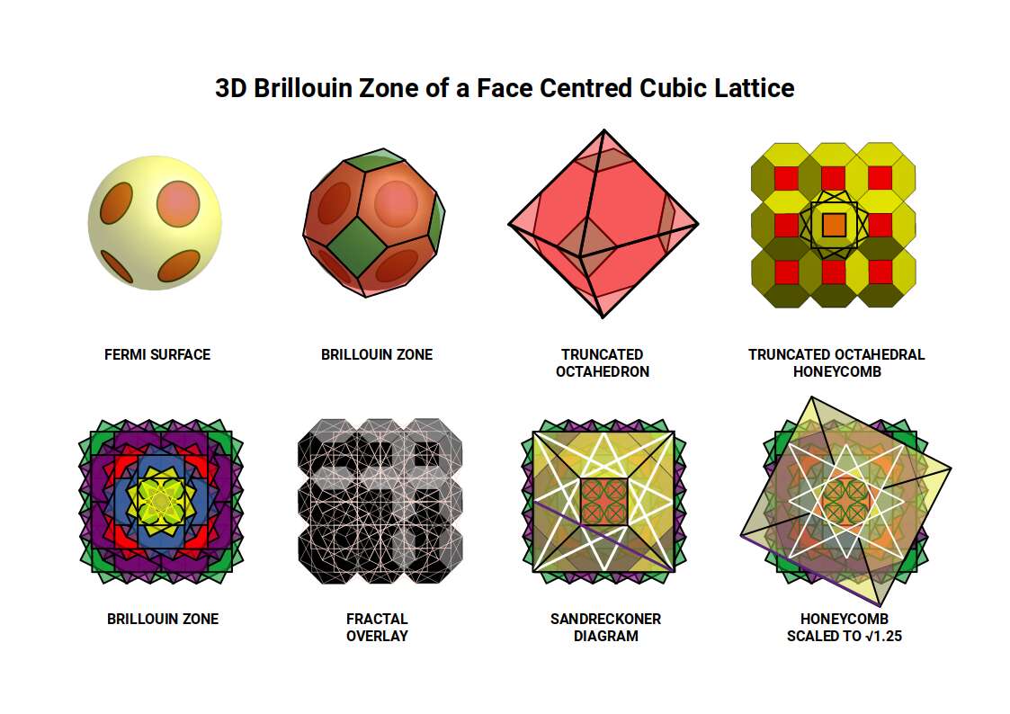
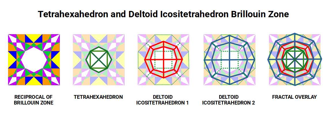
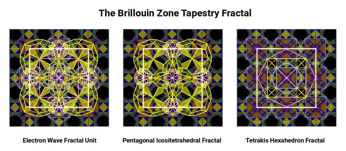
The eight-sided shape at the centre of this rotation is also the shape of the holes produced when Brillouin Zone cells are assembled into a tapestry. This shape is the orthogonal projection of the Tetrahexahedron — the dual of the Truncated Octahedron. The Brillouin tapestry is therefore formed from this reciprocal pair.
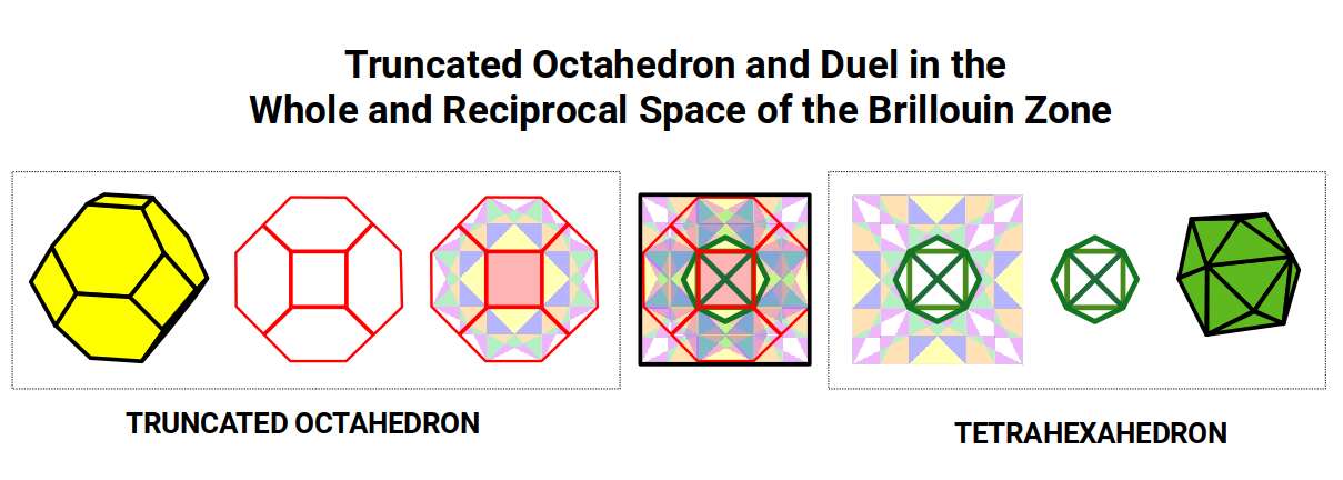
Placing the shadow projection of the Tetrahexahedron in the central space and comparing it with the projection of the Deltoid Icositetrahedron (Iron) reveals a close match. The Deltoid can be nested around the Tetrahexahedron at two scales: the first encloses the solid; the second touches the inside of the Truncated Octahedron. Together, these form a 4D template — two nested forms, just as the 4D Cube is represented by two nested cubes.
Within the Brillouin zone, the first (inner) Deltoid falls across the purple, orange and green zones, with its corners touching the corners of the yellow zone (the Rhombic Dodecahedron). When the Truncated Octahedron is superimposed, the four additional corners appear at the centres of each hexagonal face — exactly where the Fermi surfaces are located.
The second, larger Deltoid has four corners that touch the outside of the square cell (where the Rhombic Dodecahedra are centred) and four corners that reach the midpoints of the kite-shaped spaces extending at 45° angles. This produces a fractal overlay that unifies the geometry of Iron (magnetic field), the Rhombic Dodecahedral 4D cubic space, and the Tetrahexahedron (reciprocal electric field).
Turning to Chromium: its Rhombic Cuboctahedral geometry, when aligned on the Brillouin lattice with either its central square over a Truncated Octahedron face or its outer frame aligned to the cell square, does not produce a clean fit. Rotation improves the alignment but leaves the corners slightly out of registry with the grid.
After Iron, the Snub Cube forms as the radius drops to 1.35 Å. The Snub Cube's two rotated squares in its shadow projection superimpose perfectly over the sixth (purple) Brillouin Zone — but the outer shell then exceeds the Truncated Octahedron boundary. Reducing the Snub Cube so that its inner square matches the Tetrahexahedron leaves a slightly awkward outer fit. Only by rotating this smaller form is a perfect alignment achieved between the Tetrahexahedron and the Truncated Octahedron. This geometric imperfect fit offers a structural explanation for why Cobalt and Nickel are ferromagnetic to a lesser degree than Iron while having greater conductivity.
This contrast becomes fully apparent when the Pentagonal Icositetrahedron (Copper) is overlaid. Both scales match the Tetrahexahedron and Truncated Octahedron frames, and the solid can be rotated within the square cell without compromising the boundary set by the adjacent Rhombic Dodecahedra. This unique geometric freedom — fitting at multiple scales and orientations without interference — is what gives Copper its exceptional conductivity.
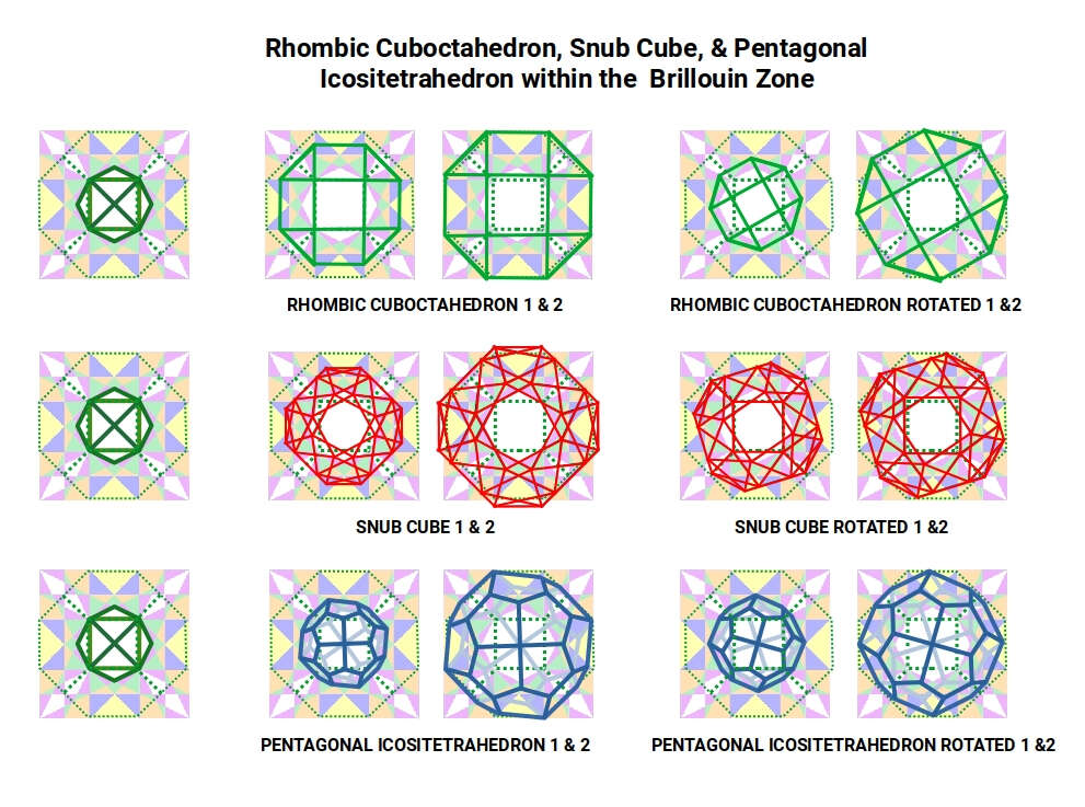
Extending the analysis to a 9-unit grid (3 × 3 cells) confirms these findings at larger scale. The Deltoid Icositetrahedron fits the centre of the grid perfectly, and can be scaled and rotated to align with the Rhombic Dodecahedra. The Snub Cube produces a clean inner match to the Tetrahexahedron but a slightly awkward outer fit. The Pentagonal Icositetrahedron matches both frames at multiple scales and rotations.
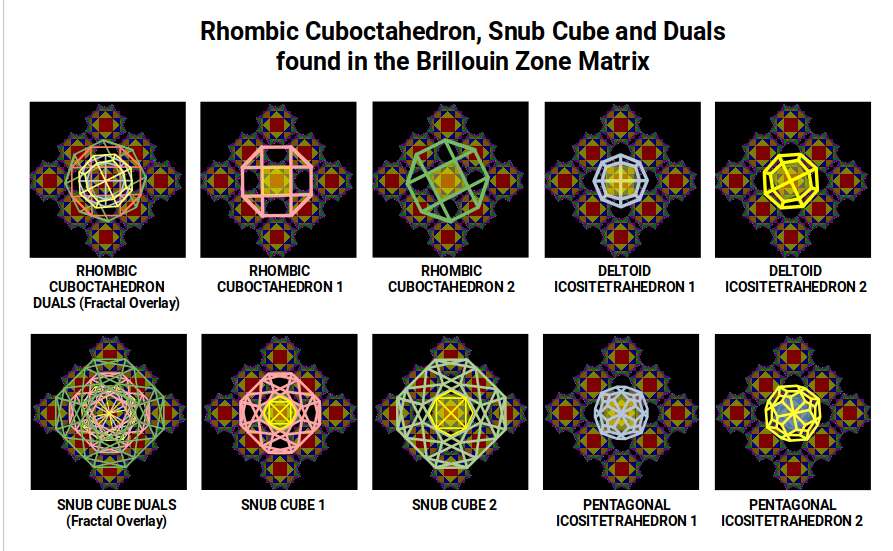
The dual geometries — Deltoid Icositetrahedron and Pentagonal Icositetrahedron — consistently produce better fits to the Brillouin zone structure than their progenitor forms. They can be scaled and rotated to align with the zones without disturbing adjacent Rhombic Dodecahedra. This pattern supports the proposal that the electromagnetic field is geometrically tuned to these rotating solids — that the lattice wave structure is, at its foundation, a geometric structure.
The Pentagonal Icositetrahedron also scales to a larger form centred over the empty inter-cell spaces in the Tetrahexahedral framework. The kite-shaped spaces between Brillouin cells are the same shape as those at the centre of the Pentagonal Icositetrahedron projection, enabling small versions of the solid to be mapped over these points. In the diagonal spaces between each cross, four larger versions can be placed with corners touching the kite shapes of the smaller versions.
Centring this fractal on the cubes rather than the holes produces a structure where the larger Pentagonal Icositetrahedra are more widely spaced — akin to the FCC structure of Copper — while the previous configuration, with four large touching Pentagonal Icositetrahedra surrounding a smaller central one, is more indicative of the BCC structure.
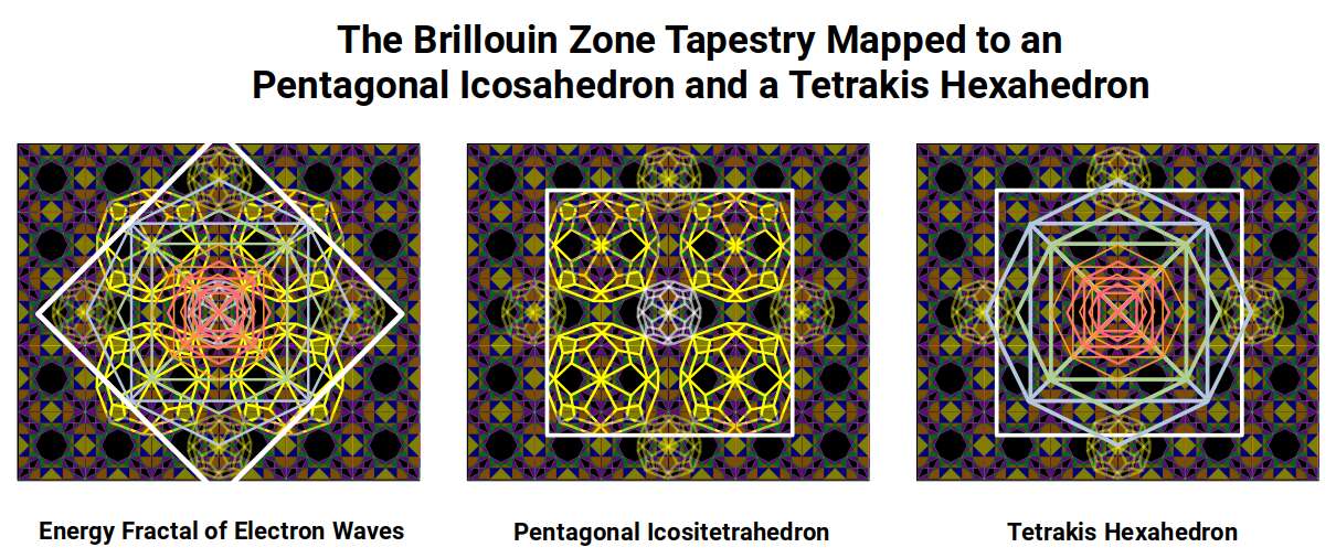
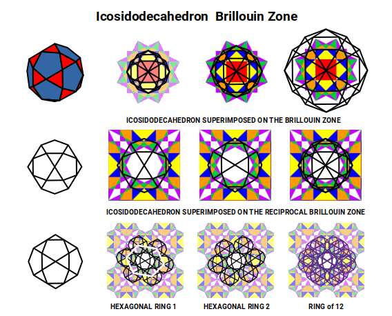
Finally, the Icosidodecahedron — whose 30 corners are assigned to the neutron count of several D-orbital elements including Iron and Nickel — produces a shadow projection that, when two orientations are superimposed at 90°, closely resembles the Pentagonal Icositetrahedron. Six of these can be arranged in a ring around a central one, producing a hexagonal plane — the blueprint for the F-orbital arrangement in Atomic Geometry. Within this fractal structure, the forms of S, P, D and F orbitals all become identifiable.
Dual Transformations and the Electromagnetic Field
Having identified the geometries of Iron and Copper within the Brillouin zone structure, we can examine what happens to the relationship between the Cube and Octahedron — the foundational solids of D-orbital and P-orbital geometry — as the D-orbital sequence progresses.
In the Snub Cube, the centre of each square face becomes the corner of the dual. These new corners are the corners of an Octahedron, which defines the out-sphere of the dual. The Cube is effectively reduced in size as the Octahedron grows to prominence within the solid.
In the Rhombic Cuboctahedral model of the D-orbitals, a unit Cube can be nested inside with its corners touching the triangular faces. When the Deltoid Icositetrahedron forms (Iron), the mid- and in-spheres become 1.3 Å and 1.22 Å respectively — matching the out-sphere of the √2 Cube also embedded in the structure. The Octahedron formed has a side of roughly √2, compounding perfectly with the √2 Cube to produce the Rhombic Dodecahedron — the same geometry as the BCC Brillouin zone of Iron. Iron's atomic geometry and its reciprocal lattice geometry are one and the same.
As the Snub Cube forms (Cobalt onwards, radius 1.35 Å), the Octahedron diminishes slightly, and the ferromagnetic properties weaken. The mid- and in-spheres reduce to 1.24 Å and 1.157 Å; the mid-sphere of the Rhombic Dodecahedron is close to 1.154 Å, providing the size differential between the second P-orbital average radius (1 Å) and the third (1.54 Å).
When the Snub Cube transforms into the Pentagonal Icositetrahedron (Copper), the Octahedron grows again. Its mid-sphere becomes 0.94 Å; when truncated, its out-sphere equals 1, aligning with the Cuboctahedron in the original D-orbital model. The Truncated Octahedron — the FCC Brillouin zone of Copper — is the direct product of this geometric transformation.
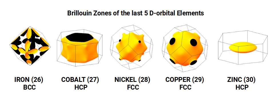
Examining the Brillouin zones of the last five D-orbital elements confirms this geometric picture. Iron produces the exterior frame of an Octahedron — a profile unique among elements. Zinc (30), with 30 protons aligned to the Icosidodecahedron's 30 corners, shifts the lattice toward the hexagonal close-packed (HCP) structure. Although Zinc shares the Pentagonal Icositetrahedral geometry of Copper, the Icosidodecahedral influence of its proton count redirects it to the HCP arrangement, which does not support the same level of conductivity.
Conclusion
Ferromagnetism and electrical conductivity are not incidental properties of a handful of elements. They are geometric consequences of the precise polyhedral forms that the proton and nucleon counts of those elements produce — forms that determine how atoms pack into lattices, how those lattices interact with electron waves, and what wave structures propagate through the resulting reciprocal space.
The theory of Atomic Geometry provides the following specific findings, each with predictive precision not available in the standard model:
- Iron is ferromagnetic because the Deltoid Icositetrahedron allows adjacent atoms to rotate in the same direction (corner-to-corner contact), unifying quantum spin across the lattice.
- Chromium and Manganese are antiferromagnetic because their Rhombic Cuboctahedral and Cuboctahedral geometries produce face-to-face lattice contact, forcing neighbouring atoms into opposing rotations.
- Cobalt and Nickel are weakly ferromagnetic because the Snub Cube geometry creates gaps between lattice atoms that partially permit co-rotation — but the fit to the Brillouin zone structure is imperfect compared to Iron.
- Copper is an exceptional conductor because the Pentagonal Icositetrahedron fits the Truncated Octahedral Brillouin zone of the FCC lattice at multiple scales and orientations simultaneously, a geometric freedom unique in the D-orbital set.
- The magnetic field is governed by the Silver Ratio (√2); the electric field by the Golden Ratio (Φ). The Tribonacci constant (η) bridges the two, appearing in the geometry of both the Deltoid Icositetrahedron (Iron) and the Pentagonal Icositetrahedron (Copper), and in the ratio between the ferromagnetic and conductive domains.
- Magnetic domain geometry follows the Rauzy fractal of the Tribonacci constant — a pattern not previously identified in a physical system.
- Negative N-bonacci waveforms generated from the atomic numbers of Iron and Copper produce outputs resembling Bloch electron waves, suggesting a new and computationally accessible alternative to the Schrödinger approach for modelling electromagnetic propagation in lattices.
The geometric model presented here is also the only framework that accurately predicts the experimentally determined atomic radii of the D-orbital elements and provides a principled geometric rule for the paramagnetic and diamagnetic behaviour of all 81 stable elements.
The implications extend beyond classification. By understanding the geometric principles that govern why certain lattice structures produce magnetic or conductive fields, it becomes possible to design new materials — Perovskite-like adaptive composites and beyond — by deliberately engineering the geometric relationships between their component atoms. This opens a path toward a new era of solid-state physics in which materials are designed geometrically rather than discovered empirically, with direct relevance to challenges such as high-temperature superconductivity and Boltzmann Tyranny in computing.
FAQ
I was taught that electrons are particles travelling down a wire. Is that wrong?
The classical Drude model of electron flow has been known to be incomplete for over a century. A more accurate description is provided by Bloch's Theorem, which treats electrons as waves propagating through a crystal lattice. This wave model is essential for explaining transistors, quantum tunnelling, and the precise behaviour of conductors — effects that the particle model cannot account for. In 4D Aether theory, quantum spin is attributed to the 4D rotation of the atom, making a wave-only model of electricity both coherent and self-consistent.
Why are Iron, Cobalt and Nickel ferromagnetic when other D-orbital elements with similar electron configurations are not?
Standard theory ascribes ferromagnetism to unpaired electrons, yet elements such as Ruthenium and Osmium share the same unpaired electron count as Iron without displaying ferromagnetic properties. Atomic Geometry offers a structural answer: the 26 protons of Iron define the Deltoid Icositetrahedron, whose corner-to-corner lattice spacing allows adjacent atoms to rotate in the same direction, aligning their quantum spins. Chromium and Manganese, by contrast, adopt geometries whose flat faces interlock like meshing cogs, forcing alternating spin orientations and producing antiferromagnetism.
What is the Tribonacci constant, and why does it appear in magnetic and conductive elements?
The Tribonacci constant (η ≈ 1.839) is derived from a number series in which each term is the sum of the three preceding terms, analogous to the way the Fibonacci series produces the Golden Ratio. It is encoded in the geometry of the Snub Cube — the form ascribed to Cobalt and Nickel — and in the ratio of the two edge lengths of the Deltoid Icositetrahedron (Iron) and the Pentagonal Icositetrahedron (Copper). The relationship between the most ferromagnetic element (Iron) and the most conductive (Copper) differs by exactly a factor of the Tribonacci constant, suggesting a deep geometric link between magnetic and electric fields.
Can Atomic Geometry predict which elements are paramagnetic or diamagnetic?
Yes — with considerably greater accuracy than electron-pairing rules alone. As a general principle, elements whose geometry is based on the Octahedron (P-orbital elements) tend to be diamagnetic, while those based on the Cube or Cuboctahedron (D-orbital elements) tend to be paramagnetic or ferromagnetic. Exceptions, such as oxygen and aluminium, can be explained by the nucleon counts that govern their specific geometric forms. This geometric rule applies consistently across all 81 stable elements.