D-Orbital Geometry - Part 3

Introduction

The 3rd set of D-orbitals is the last to form stable elements. Understanding why requires completing a dimensional progression begun in the two previous parts of this series.

In D-orbital Geometry Part 1, we established that the 1st D-orbital set (elements 21–30) maps onto the Rhombic Cuboctahedron — a geometry that encodes the 4D hypercube through the Silver Ratio. The two main radii of that set (1.35Å and 1.4Å) are produced by the in- and out-spheres of this solid. In Part 2, the 2nd D-orbital set (elements 39–48) revealed a 5D structure governed by the Truncated Cube, which orients two Rhombic Cuboctahedra at the Silver Ratio. At the midpoint of that set, the geometry transitions through the Icosidodecahedron into the Golden Ratio — a shift that renders Technetium (43) geometrically unstable and therefore radioactive. After this, the 2nd set returns toward octahedral forms as it completes.

Part 3 completes the picture. The 3rd D-orbital set (elements 70–80) maps onto the Great Rhombic Cuboctahedron, which extends the cubic sequence into the 6th dimension. The outer geometric boundary is sealed by the Rhombic Triacontahedron — the template for the 6D hypercube — and the progression terminates when the atomic radius reaches the Phi ratio. This is not merely the end of the D-orbitals: it is the geometric reason why the stable periodic table itself ends. The full theoretical context is developed in the Atomic Geometry theory.

Key takeaways

The third D-orbital set (elements 70–80) is governed by the Great Rhombic Cuboctahedron and bounded by the Rhombic Triacontahedron (the template for 6D hypercubic space), with atomic radii clustering at 1.35 Å and 1.45 Å.
The stable periodic table terminates at Bismuth (83) with a radius of approximately 1.6 Å — exactly the Golden Ratio and the geometric boundary where 6D hypercubic space completes, preventing further stable elements beyond this point.
The three D-orbital sets encode a dimensional progression: the 1st set maps 4D geometry, the 2nd maps 5D geometry, and the 3rd completes the 6D structure — a sequence that explains the periodic table's structure through dimension rather than energy alone.

3rd D-orbital set

The 3rd D-orbital set runs from elements 70 to 80, forming in the 5th shell directly after the F-orbitals complete the 4th shell. The first element, Lutetium (70), exhibits a radius of 1.75Å, the same as the preceding F-orbitals. Subsequently, the elements decrease in radius: 1.55Å for Hafnium (71), 1.45Å for Tantalum (72), and then Tungsten (73) and Rhenium (74) both at 1.35Å. This completes the first half of the D-orbital set.

Similar to the 2nd D-orbital set, the 6th element, Osmium (76), exhibits a smaller radius of 1.3Å. After this the orbital radius increases to 1.35Å for the next three elements. The final element, Mercury (80), exhibits a slightly anomalous radius of 1.5Å. The 8th and 9th elements, Platinum (78) and Gold (79), both exhibit anomalies in their electron configuration, with only a single S-orbital in the outermost shell.

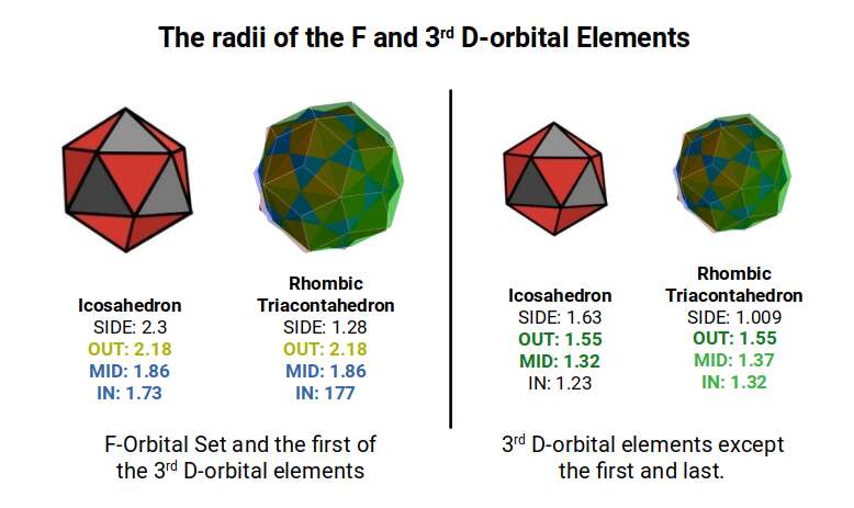
Except for Mercury (80), we can map the evolution of these radii through the out, in, and mid-sphere of two Rhombic Triacontahedra. The first is derived from the Icosahedron with a side length of 2.3Å, and the second from an Icosahedron with a side of 1.6Å. In our examination of the 2nd D-orbital set, we saw how these lengths are derived from a Cuboctahedron with an out-sphere of 1.15Å that doubles to 2.3Å as it transitions through the Jitterbug. The second radius of 1.61Å relates to the Golden Ratio, which appears as the 2nd D-orbital set completes.

Diagram mapping F- and D-orbital radii to the spheres of two Rhombic Triacontahedra — From the perspective of geometry, the final orbitals centre around the mid-sphere of the smaller Rhombic Triacontahedron. This forms the template for the 6D hypercube.

As with the previous D-orbital sets, we can see what emerges when we expand a Cuboctahedron through the Dodecahedron transformation. The 4th P-orbital set (elements 49–54) exhibits a radius of 1.41Å, or √2. This means that when transformed through the Dodecahedron, the final Cuboctahedron will exhibit a larger side length of 2. Notice this is roughly the same size as the average radius of the 2nd P-orbital set, which begins with a Cuboctahedron with a side of 1. When transformed through the Rhombic Dodecahedron and the Jitterbug, this also produces a new Cuboctahedron with a side length of √2.

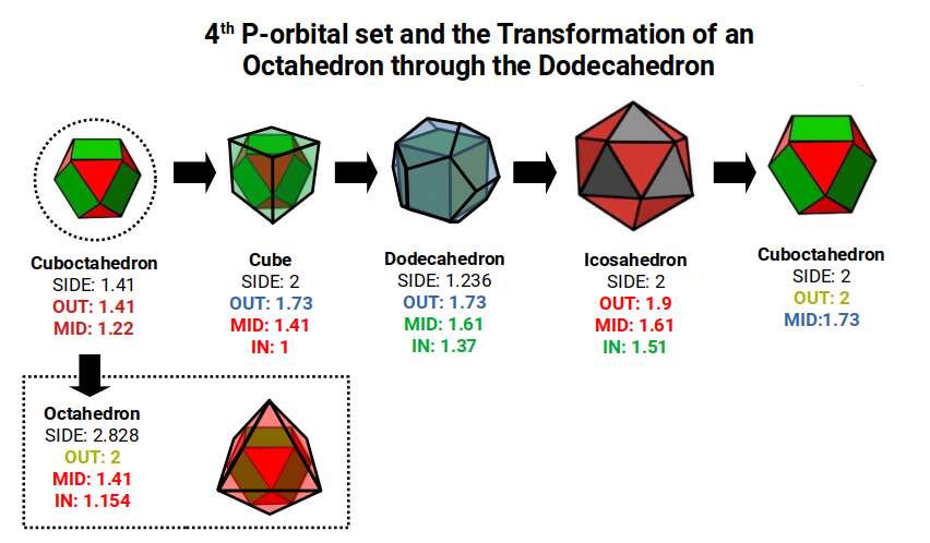
Cuboctahedron with side √2 transforming through the Dodecahedron into a larger Cuboctahedron — The Cuboctahedron (left) with a side of 1.41 (√2) transforms through the nested relationship of the cube, dodecahedron, and icosahedron, which finally expands through the Jitterbug into a Cuboctahedron (right) with sides √2 greater.

The Cuboctahedron can produce a compound of the Cube and Octahedron, defining the foundational radii of the 2nd, 3rd, and 4th P-orbital sets: 1Å, 1.154Å, and 1.41Å respectively. The Dodecahedron that sits around the Cube exhibits a mid-sphere of 1.61, representing the largest D-orbital elements, Scandium (21) and Silver (47). The in-sphere roughly defines the radius of 1.35Å found in the majority of D-orbitals. The Icosahedron exhibits an in-sphere of 1.5, which is the radius of Mercury (80), the last D-orbital element.

After this, only 3 more P-orbitals form before the radioactive elements begin. The first, Thallium (81), exhibits a radius of 1.9Å found in the out-sphere of the Icosahedron. This is followed by Lead (82), sometimes quoted at 1.8Å or 1.75Å — the latter found in the out-sphere of the Dodecahedron. Finally, the last stable element on the periodic table, Bismuth (83), has a radius of 1.6Å, found in the mid-sphere of both the Icosahedron and Dodecahedron, the point at which the Rhombic Triacontahedron is formed.

As the Icosahedron has a side of 2, its mid-sphere is the Golden Ratio (Φ), 1.618. The side of the Dodecahedron is 2÷Φ, and the Rhombic Triacontahedron has a side of 1. The atoms on the stable periodic table therefore terminate once at the Phi ratio, in the mid-sphere of the Triacontahedron — the template for the 6D hypercube.

We can compare the geometric model to the Bohr and experimental datasets. As with the other D-orbital elements, the Bohr model overshoots the radii of the D-orbital set. Furthermore, as the 5th P-orbitals form, the Bohr radius drastically undershoots the experimental values. The existing model has no explanation for the sudden increase in these last P-orbital sets, nor why only 3 out of 6 should be stable. In the final elements, there are a total of 5 electrons in the outermost shell. This matches the pentagonal geometries formed by the Icosahedron and Dodecahedron. Similarly, the 5th element in the 2nd D-orbital set is unstable as the set transitions from 4D to 5D — only this time the D-orbital structure moves into the 6th dimension.

The Rhombic Triacontahedron and the Icosidodecahedron

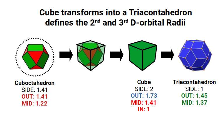
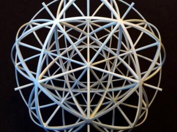
The Rhombic Triacontahedron defines the blueprint for the 6D hypercube in the same way that the Rhombic Dodecahedron forms the blueprint for the 4D cube. Whilst it can be created by compounding the Dodecahedron and Icosahedron, it can also be formed through a process similar to the Jitterbug. Each square face of the cube is divided in half and expanded to create two new triangular faces. This can be accomplished in exactly two different orientations, with the split running through the horizontal or vertical of the cube's face. The new vertex created between the two triangles is also orientated at 90°, mirroring the orientations found in the Star-Dodecahedron. This gives the Rhombic Triacontahedron two distinct possibilities in terms of orientation.

Animated transformation of a cube into the Rhombic Triacontahedron — A cube with side length 2 transforms into a Rhombic Triacontahedron by halving each face into two triangles, producing out- and mid-sphere radii of 1.45Å and 1.37Å respectively.

A cube with a side length of 2 has an in-sphere of 1 and a mid-sphere of 1.41, which is the radius of the 2nd and 4th P-orbital sets. When transformed into a Rhombic Triacontahedron, each side is halved in length. This produces a Triacontahedron with an out-sphere of 1.45 and a mid-sphere of 1.37. These two radii predominate across the D-orbital sets, beginning with Iron (26). The entire second half of the 1st D-orbitals conforms to a radius of 1.35Å. The start and end of the 2nd D-orbital set sees many elements conform to 1.35Å or 1.45Å. In the 3rd D-orbital set, the radius of the cube (1.41Å) is absent; the elements fall from 1.45Å to 1.35Å. What emerges is that the 6D cube begins to form around this area, which is also where the D-orbital sets are generally composed.

Diagram showing a cube transforming into the Triacontahedron and defining the 2nd and 3rd D-orbital radii — The cube (side 2) transforms into the Rhombic Triacontahedron, whose out- and mid-sphere radii of 1.45Å and 1.37Å define the predominant radii of the 2nd and 3rd D-orbital sets.

As the Triacontahedron comprises a compound of an Icosahedron and Dodecahedron, it naturally inherits the pentagonal geometries that exhibit the Golden Ratio. If its side length is 1, the out-sphere that encompasses it will be Phi. The difference between the out- and mid-sphere is √1.25, which when 0.5 is added also equals Φ. Just as the Icosahedron exhibits a pentagonal prismal mid-section, the same is inherited by the Rhombic Triacontahedron. However, due to the intersection of the Dodecahedron, a second pentagonal plane can be found internally. These two types of pentagon exhibit the side lengths of the Icosahedron and Dodecahedron, which when compounded are in a 1:Φ ratio.

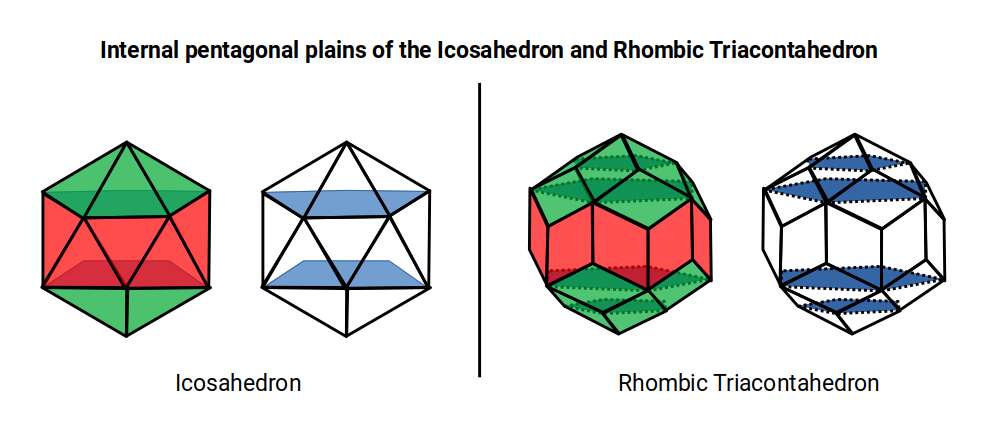
Comparison of the pentagonal planes found in the Icosahedron and Rhombic Triacontahedron — The Icosahedron (left) exhibits a single pentagonal mid-section. The Rhombic Triacontahedron (right) inherits this and adds a second pentagonal plane from the Dodecahedron — the two pentagons are in a 1:Φ ratio.

The Atomic Geometry theory suggests the Icosahedron forms a double torus found in the F-orbital set, denoted by the fact that it is comprised of a pentagonal prism as its centre. The Rhombic Triacontahedron extends this notion, adding another layer from the pentagonal sides of the Dodecahedron. Similarly, the final D-orbital torus completes a set of 3 torus fields, which can be represented in its structure.

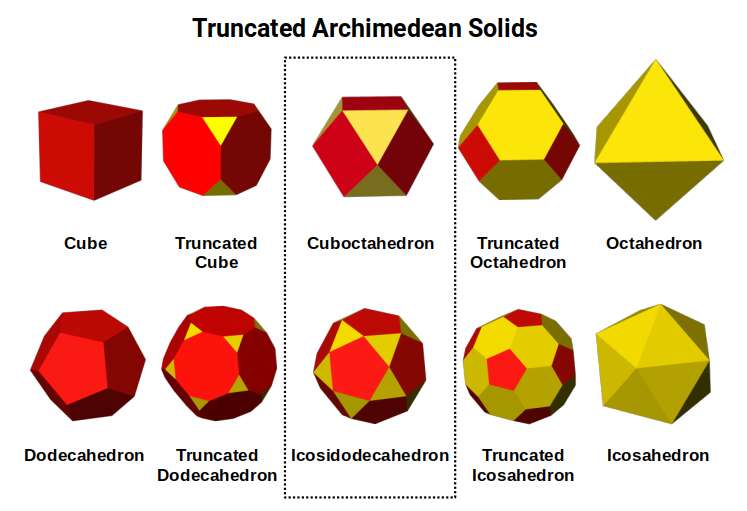
The Rhombic Triacontahedron also has a dual: the Icosidodecahedron. This solid can be formed by truncating the corners of a Dodecahedron or Icosahedron, analogous to the truncation of a Cube or Octahedron that creates the Cuboctahedron.

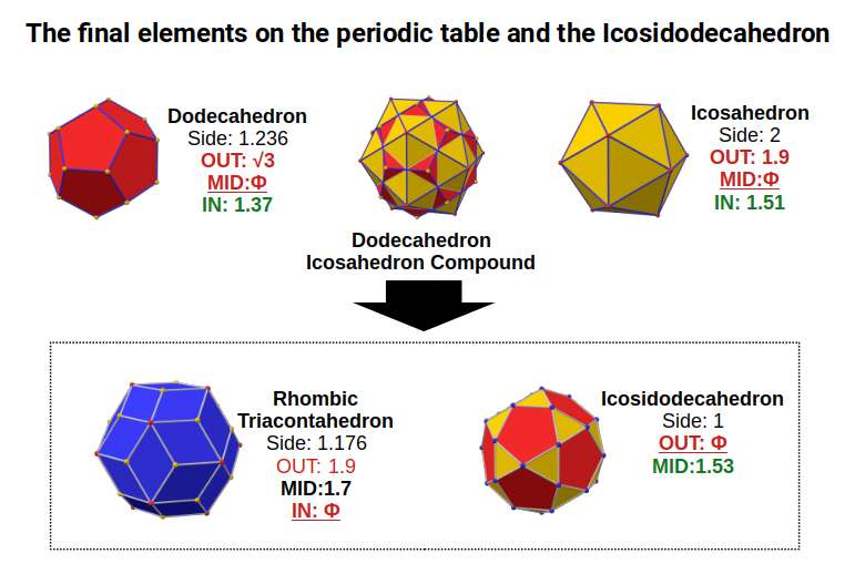
Comparison of truncated Archimedean solids showing the Cuboctahedron and Icosidodecahedron as dual counterparts — Truncating the corners of a Cube or Octahedron produces the Cuboctahedron; truncating the Dodecahedron or Icosahedron produces the Icosidodecahedron — its pentagonal analogue.

When we examine the structure of a compound of the Icosahedron and Dodecahedron generated by the 4th P-orbital set, we find that the Rhombic Triacontahedron exhibits an out-sphere of 1.9, the radius of the initial 5th P-orbital element. The final element, Bismuth, has a radius of Φ, found throughout the set and also as the out-sphere of the Icosidodecahedron. Note that this polyhedron has a side length of 1 — exactly half that of the Icosahedron from which it was derived. Its in-sphere has a value of 1.53, close to 1.55Å, the experimentally determined radius for many of the D-orbital elements.

The Icosidodecahedron mapped against the radii of the last stable elements on the periodic table — The Icosidodecahedron (side length 1) produces an out-sphere of Φ and an in-sphere of 1.53. These radii correspond to Bismuth (83) and the general D-orbital radius of 1.55Å respectively.

The radius of 1.55Å first appears for Zirconium (40), after which the 2nd D-orbital anomalies begin, leading to the instability of Technetium (43). As this set transitions into the 4th P-orbitals, the radius of Silver (47) at 1.6Å, Cadmium (48) at 1.55Å, and the first P-orbital element Indium (49) are also found.

Both the Icosidodecahedron and Rhombic Triacontahedron, transformed from the cube previously, exhibit the same side length of 1. Between them we are able to define the radii of the majority of D-orbital radii as well as many of the S- and P-orbital elements.

There is also a relationship between the Icosidodecahedron, Icosahedron, and Octahedron. An Octahedron can be positioned inside an Icosahedron so that its corners touch the midpoints of 6 of its edges. As the Octahedron grows in size, each of its corners pushes outward. Inside the Icosahedron, 3 golden rectangles can be composed with a side length ratio of 1:Φ. The longer side corresponds to the diagonal across the internal pentagram.

As the Icosahedron has 30 sides, 5 Octahedra can be nested in 5 different orientations, just like the 5 cubes in the Dodecahedron. If the Octahedra is expanded in size, its corners distort the shape of the Icosahedron, transforming it into an Icosidodecahedron. In doing so, the internal planes are transformed into 3 golden cubes with a ratio of 1:Φ:Φ². As there are 5 possible orientations for the Octahedron, there are also 5 types of Icosidodecahedra that can be created from this transformation.

Animated transformation of an Octahedron inside an Icosahedron into an Icosidodecahedron — Expanding an Octahedron nested within an Icosahedron distorts the triangular faces into pentagons, transforming the Icosahedron into an Icosidodecahedron. The internal golden rectangles become 3 golden cubes in ratio 1:Φ:Φ².

The Icosidodecahedron and E8 Geometry

The geometric relationships explored above do not stop at 6 dimensions. The Icosidodecahedron connects this model to a far larger geometric structure — and understanding why clarifies the deeper architecture behind the atomic boundary.

The Icosidodecahedron has been recognised as a projection of the E8 geometry. This matters here because E8 is the geometry underlying string theory's unification of fundamental forces — and the same form appears naturally at the boundary of stable matter. In Atomic Geometry, this is not coincidental: the same geometric constraints that produce the 6D hypercube also project into 8D as the E8 lattice, suggesting that the boundary of stable matter is a direct consequence of the dimensional limits encoded in these forms.

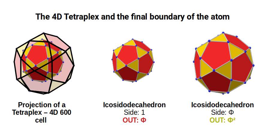
Concretely: the E8 polytope is an 8th-dimensional object with 240 vertices. It can be projected in 4D as two 600-cells, called the Tetraplex. Based on the Icosahedron, this 4D polytope is made of tetrahedral cells and has 120 vertices exactly. When two combine, the number of vertices doubles, producing the E8 form found at the heart of the E8 theory.

The Tetraplex is a 4D object which, like the 4D cube, can be constructed from two nested polyhedra. This is best applied to a pair of nested Icosidodecahedra. By adjusting some of the vectors to be in golden proportion to the others, each form can be separated by a distance of Φ.

Animated rotation of the 4D 600-cell — Rotation of the 4D 600-cell (Tetraplex), constructed from tetrahedral cells with 120 vertices.

Animated projection of the 600-cell as two nested Icosidodecahedra — The 600-cell projected as two nested Icosidodecahedra, with vertices separated by the Golden Ratio Φ.

Diagram showing half a 600-cell forming the Icosidodecahedra — Half a 600-cell forms the Icosidodecahedron. The small protruding points at the centre of each pentagonal face connect to the second half of the form in higher dimensions.

Each Icosidodecahedron exhibits 30 corner points — the number of D-orbital electrons across the 3 shells. Each point is therefore connected to each other through the Golden Ratio. In the model of half a 600-cell, the midpoint of each pentagonal face has a small protruding point. In higher dimensions, these connect to the second half of the form.

Returning to our geometric model of the atom, an Icosidodecahedron with a side of 1 produces an out-sphere of Φ and a mid-sphere of 1.53. We previously associated these values with the radii formed at the end of the 2nd set of D-orbitals leading onto the 4th P-orbital set up to the noble gas Xenon (54). After this, Caesium (55) exhibits the first S-orbital in the 6th shell. This element has a radius of 2.6Å — the largest of any on the periodic table — very close to 2.618, or Φ². As the 5th P-orbitals begin to fill this shell, only 3 electrons form elements, bringing the total to 5 (3P and 2S-orbitals). At this point the radius falls, with Bismuth (83) exhibiting a radius of 1.6, or Φ. Therefore Caesium (55), which starts to fill the 6th shell, and Bismuth (83), which ends it, exhibit a Φ relationship — perfectly expressed by the projection of a Tetraplex through two nested Icosidodecahedra.

Diagram of the 4D Tetraplex mapping the Phi relationship between Caesium and Bismuth — The 4D Tetraplex (projected as two nested Icosidodecahedra) maps the Φ relationship between Caesium (55) at 2.6Å ≈ Φ² and Bismuth (83) at 1.6Å ≈ Φ — defining the outer boundary of the stable atom.

This notion of Phi which creates the Golden Ratio is well known in sacred geometry. What is less often recognised is that Phi has a sibling — the Silver Ratio — which also produces a 6D hypercubic model of the atom.

The Great Rhombic Cuboctahedron

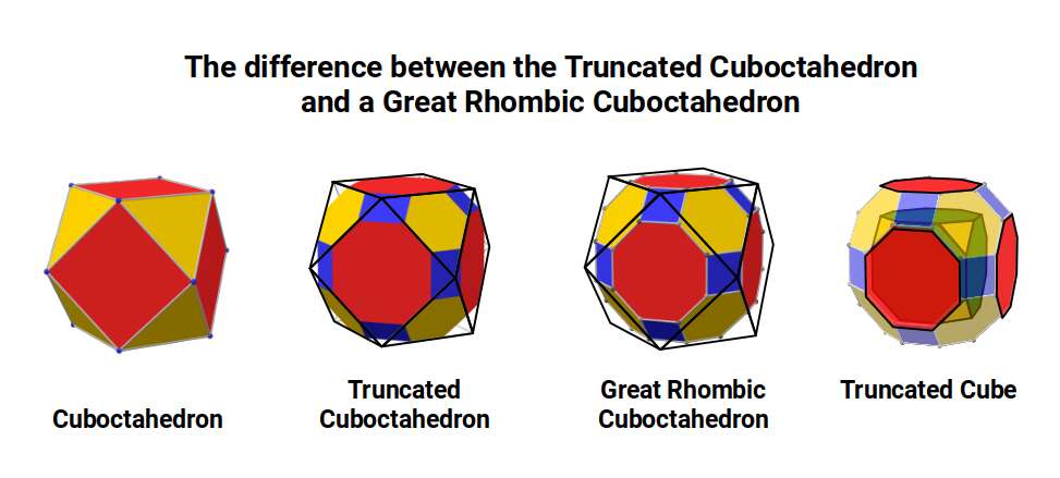
The Truncated Cube has a larger counterpart called the Great Rhombic Cuboctahedron. By moving the octagonal faces away from the centre, the space between each one becomes sufficient to add a square between each one. At this point the corners become composed of hexagons instead of the triangular faces found in the Rhombic Cuboctahedron.

In our geometric model of the atom, the Truncated Cube appears in the 2nd D-orbital shell, producing the slightly enlarged radius of 1.47Å. Around this we can place a Great Rhombic Cuboctahedron, whereby its mid-sphere meets the out-sphere of the Truncated Cube. This produces a slightly larger out-sphere of 1.51, which is almost exactly the radius of Mercury (80). The preceding elements all have a radius of 1.35Å, found in the mid-sphere of the Rhombic Triacontahedron. Once the set completes, there is a large jump in radius to 1.5Å, just as the last D-orbital completes. The radius of the out-sphere of the Truncated Cube appears only once, at the 3rd element Tantalum (73), just as the 3 cross-shaped D-orbitals form. Therefore, the mid- and out-sphere of the Great Rhombic Cuboctahedron appear in both the 3rd and 10th shells.

Around the Great Rhombic Cuboctahedron, we can place a Cuboctahedron so that the out- and mid-spheres of each solid align. The Cuboctahedron produces a new out-sphere of 1.74, extremely close to the radius of the smaller F-orbital elements at 1.75Å. In Atomic Geometry, we represent the 4 hexagonal-shaped F-orbitals within the structure of the Cuboctahedron.

Alternatively, we can align the out-sphere of the Great Rhombic Cuboctahedron with the in-sphere of a cube. This produces a mid- and out-sphere of 2.13 and 2.61, equating to the radius of the last pair of stable S-orbitals: Caesium (55) at 2.6Å and Barium at 2.15Å, which form the 6th shell.

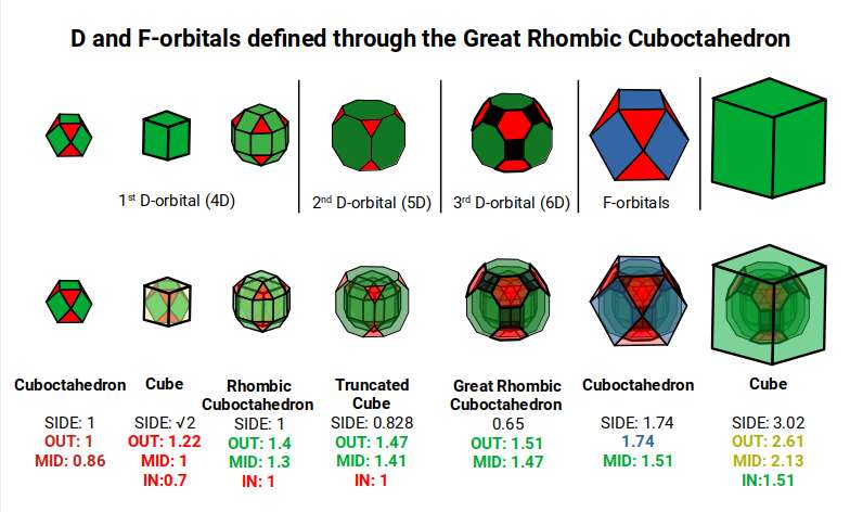
Diagram showing how the Great Rhombic Cuboctahedron defines the radii of D- and F-orbitals — The Great Rhombic Cuboctahedron nested within a Cuboctahedron defines the F-orbital radius (1.74Å). When its out-sphere is enclosed in a cube's in-sphere, the resulting radii correspond to Caesium (2.6Å) and Barium (2.15Å).

This geometric model expresses a cubic perspective of the D-orbital sets. Including the Snub Cube with an out-sphere of 1.35, all D-orbital radii are expressed in this model. The smaller geometries to the left of the set also provide the radius of many of the 1st P-orbital elements. As the geometries build into the 2nd D-orbital set, the Truncated Cube introduces a slightly larger radius of 1.47. Finally, as the 3rd set completes, Mercury appears as the only D-orbital element with a radius of 1.5Å.

This model expresses the nature of the hypercube as it expands through dimensional space. The 1st D-orbital set contains two cubes with side lengths 1 and √2, indicative of a 4D hypercube. The Truncated Cube adds another layer, producing 3 cubes as found in a 5D hypercube. The final layer is produced by the Great Rhombic Cuboctahedron, which adds a 4th cube to the set, completing the model of a 6D hypercube. This final boundary is also expressed as the Rhombic Triacontahedron, which forms the blueprint for the 6D cube in the same way that the Rhombic Dodecahedron produces the 4D hypercubic template.

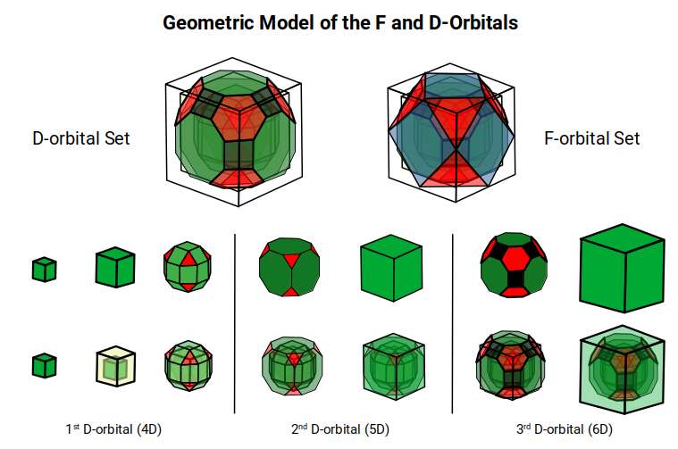
Cubic perspective diagram showing 4 nested cubes corresponding to the 4D, 5D, and 6D hypercubic D-orbital sets — The cubic perspective of the D-orbital sets: four nested cubes — sides 1 and √2 (4D), plus Truncated Cube (5D), plus Great Rhombic Cuboctahedron (6D). The Rhombic Triacontahedron forms the outer boundary.

In the model above, 4 cubes are indicative of a stereographic projection of a 6D hypercube. In the 1st D-orbital set, two cubes are found with sides of 1 and √2. This 4D cubic structure is oriented by the Rhombic Cuboctahedron. The Truncated Cube is found in the 2nd D-orbital set, which can topologically transform into the Icosidodecahedron, producing a 5D hypercubic arrangement inside the Dodecahedron.

The final D-orbital set is represented by the Great Rhombic Cuboctahedron. This has a special relationship to the Rhombic Cuboctahedron: 12 cubes can be placed on the inside of the square faces of the Great Rhombic Cuboctahedron, aligning perfectly with the square faces of the Rhombic Cuboctahedron. This produces a uniform distance between the polyhedra and its side length — a projection of a uniform polytope in higher-dimensional space.

With a side length of 1, the Rhombic Cuboctahedron exhibits an octagonal mid-section that measures √2+1 (the Silver Ratio) between opposite edges. Adding cubes to either the top or bottom section extends this distance to √2+2 when viewed from above, due to the 45° incline of the attached cube. When the mid-section is extended in the same manner, the distance between edges increases to √2+3. This provides an interesting extension of the Silver Ratio, based on the numbers 1, 2, and 3, as the cube expands into higher-dimensional space.

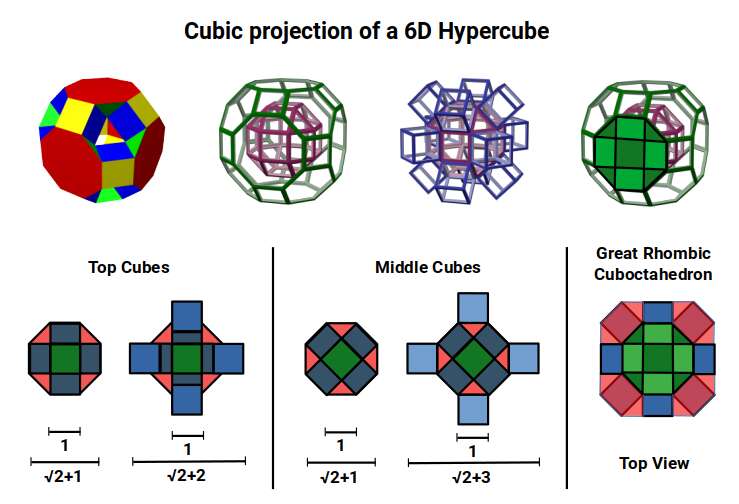
Cubic projection of the 6D hypercube showing 12 five-dimensional hypercubic cells — The 6D hypercube is formed of 12 five-dimensional (5D) hypercubic faces — the same number of cubes added to the faces of the Rhombic Cuboctahedron. Each 5D cell consists of 3 cubes governed by the Silver Ratio.

A 6D hypercube is formed of 12 five-dimensional hypercubic faces — the same number of cubes added to the faces of the Rhombic Cuboctahedron. Examining the structure of this cell, it consists of two cubes separated by a gap: the outer cube extruded from the surface of the Rhombic Cuboctahedron, and the inner cube formed from the small cube at the centre that when exploded produces the Rhombic Cuboctahedron. A 3rd cube can be added to the inside, filling the space between them. This will either overlap the centre cube or, when attached to its face, overspill above the surface. In either state the ratio of 1:√2−1 is maintained — this is the Silver Ratio, expressible as √2±1. This cubic cell is therefore comprised of 3 cubes indicative of a 5D cube, governed by the Silver Ratio. A 6D cube exhibits 12 of these 5D cells, the same number found between the Rhombic Cuboctahedron and its larger counterpart, the Great Rhombic Cuboctahedron.

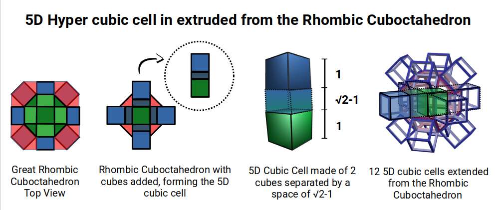
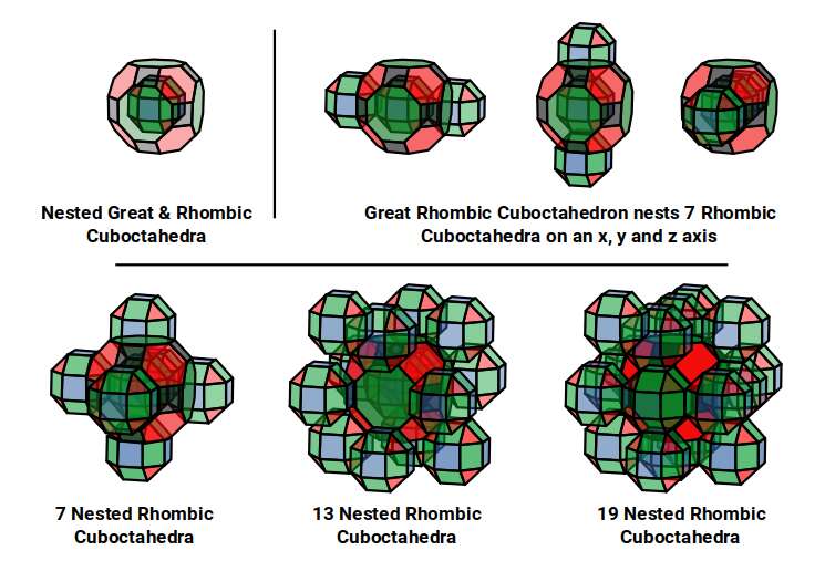
Diagram of a 5D hypercubic cell extruded from the surface of a Rhombic Cuboctahedron — A 5D hypercubic cell extruded from the Rhombic Cuboctahedron, comprising 3 cubes in a Silver Ratio relationship (1:√2−1). Twelve of these cells compose the full 6D hypercube.

The model of a 6D cube leaves space above the octagonal faces of the Great Rhombic Cuboctahedron. These can be filled with 6 more Rhombic Cuboctahedra, aligned on the x, y, and z axes. Once complete, the remaining square faces where the 5D cubic cells were formed can be filled with another 12 Rhombic Cuboctahedra, bringing the total in the set to 19, including the one at the centre of the construct.

Diagram of 19 Rhombic Cuboctahedra arranged around the Great Rhombic Cuboctahedron — The complete 6D construct: 19 Rhombic Cuboctahedra — 1 central, 6 on the octagonal faces along x/y/z axes, and 12 on the remaining square faces — arranged around the Great Rhombic Cuboctahedron.

When we separate out these two types of arrangements, we find they exhibit an Octahedral and Cuboctahedral structure — matching the geometric arrangement of the D- (and even P-) orbital sets. The Octahedral configuration can be expanded by adding more Great Rhombic Cuboctahedra to each of the 6 external Rhombic Cuboctahedra. This pattern can be extended indefinitely, leaving small cubic spaces where the 5D cells appear. The same cannot be said of the Cuboctahedral structure. These attach to the outer square faces of the Great Rhombic Cuboctahedron, which prevents the expansion of this set into infinity. This is why there are no stable D-orbital elements beyond the 3rd set — the structure is limited to the 6th dimension by its Cuboctahedral nature.

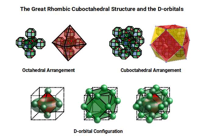
Comparison of the Octahedral and Cuboctahedral arrangements of the Great Rhombic Cuboctahedral matrix with D-orbital sets — The Octahedral arrangement (left) can expand infinitely; the Cuboctahedral arrangement (right) is self-limiting. This geometric constraint explains why the D-orbitals terminate after 3 sets.

The Octahedral P-orbitals and Cuboctahedral D-orbital geometries are further distinguished by replacing the Rhombic Cuboctahedra with 6 Truncated Cubes (5D hypercubes). These fall on the x, y, and z axes, representative of the P-orbital sets. Upon the hexagonal faces of the Great Rhombic Cuboctahedron, Truncated Tetrahedra can be placed. This produces new spaces for a set of 12 more Great Rhombic Cuboctahedra, oriented like the D-orbitals. The F-orbitals contain two star-tetrahedral orbitals in the same orientation as the Truncated Tetrahedra. This configuration can be expanded through both an Octahedral and Cubic arrangement — similar to the Rhombic Dodecahedron — filling 3D space uniformly into infinity.

First stage of the Great Rhombic Cuboctahedral structure build-up with Truncated Cubes on axial faces — Stage 1: Truncated Cubes (5D hypercubes) placed on the x, y, z axial faces of the Great Rhombic Cuboctahedron, representing the P-orbital sets.

Second stage adding Truncated Tetrahedra on hexagonal faces — Stage 2: Truncated Tetrahedra placed on the hexagonal faces, opening spaces for D-orbital-oriented Great Rhombic Cuboctahedra. The F-orbital star-tetrahedral forms share this orientation.

Third stage showing the full Octahedral and Cuboctahedral arrangement filling space — Stage 3: The full Octahedral arrangement, which can extend indefinitely into space — analogous to the P-orbital structure.

Fourth stage showing the Cuboctahedral arrangement limited by the square face geometry — Stage 4: The Cuboctahedral arrangement is self-terminating due to the square face geometry — geometrically encoding the termination of the D-orbitals at the 3rd set.

The Light Boundary

The self-terminating nature of the Cuboctahedral arrangement establishes the upper geometric limit of the D-orbitals in abstract space. But this limit also has a direct physical expression: the outer radius of the stable atomic structure corresponds, with striking precision, to the distance light travels in one attosecond. The following analysis uses the extended hypercubic model to show this relationship and map all stable atomic radii within a single coherent scale.

When considering the 6D construct produced by the Great Rhombic Cuboctahedron, the side lengths remain consistent throughout the structure. This differs from the D-orbital model presented, where the unification of mid-spheres of each solid produces a decrease in the side of each subsequent polyhedron. The Rhombic Cuboctahedron is based on a side of 1, exploded from a cube with the same edge length. The Truncated Cube is derived from a cube with a side length of 2, giving it a side of 0.828, or √8−2. Note that this is double the value of the Silver Ratio (√2−1), so it still exhibits the same qualities. The Great Rhombic Cuboctahedron has a side of 0.65, close to 2÷3 (0.666…).

When first rediscovered by Johannes Kepler, he originally called the Great Rhombic Cuboctahedron the 'Truncated Cuboctahedron'. However, due to the nature of the Silver Ratio found in the octagon and the triangular faces of the Cuboctahedron, this procedure would elongate the square faces of the Great Rhombic Cuboctahedron. Therefore, the only correct geometric procedure to form this polyhedron is to explode the faces of the Truncated Cube. A Great Rhombic Cuboctahedron will therefore have a side length that is between the longer and shorter sides of the Truncated Cuboctahedron.

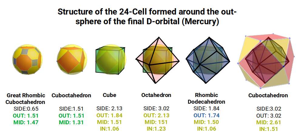
Comparison between the Truncated Cuboctahedron (Kepler's version) and the geometrically correct Great Rhombic Cuboctahedron — Kepler's 'Truncated Cuboctahedron' (left) distorts the square faces due to the Silver Ratio. The geometrically correct Great Rhombic Cuboctahedron (right) is formed by exploding the faces of the Truncated Cube, preserving all face regularity.

In our model, we enclosed the out-sphere of the Great Rhombic Cuboctahedron (1.51) in the in-sphere of a cube. This produces an out-sphere of 2.61, very close to the square of the Golden Ratio. We can also place a Cuboctahedron inside the sphere, which can be used to build the compound of a Cube and Octahedron — which in turn forms the Rhombic Dodecahedron. The Octahedron can be transformed through the Jitterbug transformation to produce an Octahedron twice the size. This shifts the ratio of the structure by 1.154, which is the difference between the 2nd and 3rd P-orbital sets. This produces a new set of radii, with the largest being the out-sphere of the large Cuboctahedron at just over 3Å. Examination of these radii reveals a striking correspondence to the size of 7 of the 12 stable S-orbital elements.

It is interesting to note that the combination of the Rhombic Dodecahedron and Cuboctahedron is analogous to the 24-cell or Octaplex, which is unique to the 4th dimension — sometimes referred to as the 6th Regular 4D shape, which in Atomic Geometry is ascribed to the F-orbitals.

The 24-cell (Octaplex) placed around the atomic structure defined by the Rhombic Dodecahedron and Cuboctahedron — The 24-cell (Octaplex) placed around the atomic structure. This 4D analogue of the combined Rhombic Dodecahedron and Cuboctahedron corresponds geometrically to the F-orbital shell.

We can call this the compressed model, as the difference between the sizes of the Rhombic Cuboctahedron, Truncated Cube, and Great Rhombic Cuboctahedron is closely spaced. This is because the Truncated Cube is derived from a cube with a side of 2.

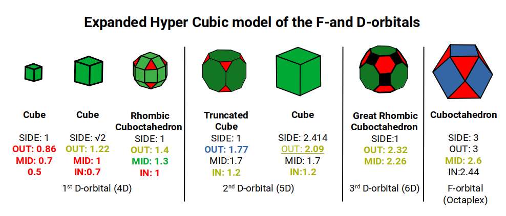
We can also produce a model whereby these 3 polyhedra exhibit the same side length, as presented in our explanation of 6D hypercubic space. The 1st D-orbital set, up to the Rhombic Cuboctahedron, remains the same. After this, the Truncated Cube is derived from a cube with a side of √2+1. This maintains the Truncated Cube's edge size at 1, producing a much larger radius of 1.77, where the F-orbital elements are found. Note that the F-orbitals appear in the 4th shell.

The Great Rhombic Cuboctahedron with a side of 1 produces a much larger circumference. The mid-sphere measures 2.26, slightly larger than 2.2Å — the radius of Potassium (19) at the start of the 4th shell. The out-sphere marks a radius of 2.32, close to the radius of Rubidium (37), which appears in the same place in the next shell up. Finally, the radius of Caesium (55) — again the first to appear in the 6th shell — is found in the mid-sphere of the Cuboctahedron.

Extended hypercubic model of the D-orbital set with all three polyhedra at the same side length — The extended hypercubic model: all three polyhedra (Rhombic Cuboctahedron, Truncated Cube, Great Rhombic Cuboctahedron) set to the same side length. The radii correspond to Potassium (2.2Å), Rubidium (2.32Å), and Caesium (2.6Å) at the opening of successive shells.

In this model, the value of the side of the Great Rhombic Cuboctahedron is tripled, as if it were truncated from the Cuboctahedron. The true size of the Cuboctahedron will be marginally larger, as found in the 24-cell compressed model. Both models converge at roughly the same point, where the Cuboctahedron has an out-sphere of approximately 3Å.

We can compare these radii to the experimentally determined results for all S-orbital elements, excluding Helium (1), whose radius of 0.25Å is easily derived from halving the first P-orbital radii. When compared to the predictions of the Bohr model, this geometric interpretation offers a much closer match to the experimental data.

The point where both datasets agree is at the radius of Magnesium (1.5Å). After this, the Bohr model increases in radius, moving away from experimentally determined values. The geometric model predicts a slightly larger radius for Strontium, which appears in the same shell as the orbital set. Strontium has a radius of 2Å, more accurately described by the out-sphere of the Cuboctahedron with the same side length — found at the end of the Jitterbug transformation of the 4th P-orbital set.

According to the Bohr radius, the size of the largest atom, Barium (56), is 2.98Å — close to the final out-sphere of the Cuboctahedron produced by both the contracted and extended hypercubic model. This value also happens to be close to the speed of light, which is 299,792,458 metres per second. When the metre is scaled to Ångströms, light takes 1 attosecond to travel the radius of the out-sphere of the Cuboctahedron, which is 10⁻¹⁸ seconds.

Presently, the limitation of speeds observed by science is 100 attoseconds. Whilst determining the detailed nature of events at this speed is beyond our present capabilities, we can use this relationship to produce a scale that denotes the radius of various atoms and forms a comparison to the geometric nature of space.

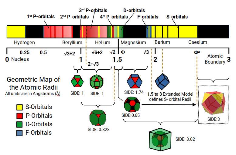
Geometric map of all atomic radii from hydrogen to barium, scaled against geometric sphere radii — A geometric map of atomic radii from zero (nucleus) to the out-sphere of the Cuboctahedron (≈3Å). The scale reveals structural groupings corresponding to each orbital set and the geometric solids that define them.

The scale starts at zero, where the atomic nucleus is found. The smallest atom, Hydrogen, has a radius of 0.25Å. There is then a space of 0.25Å before the next smallest atom, Fluorine (9) in the 1st P-orbital set — forming a 1:2 ratio of space. After this, the next smallest atoms are in the 2nd P-orbital set. The space between the largest of the 1st P-orbitals and the smallest of the 2nd is defined by the mid- and out-sphere of the Cuboctahedron with a side of 1.

The 2nd and 3rd P-orbitals overlap, but exhibit a general radius of 1Å and 1.154Å respectively. Between them sits Beryllium (4), with a radius of 1.06Å. When multiplied by the 3rd P-orbital radius (1.154), the result produces the size of the Helium atom (√6÷2). From the first 3 P-orbital sets, only Gallium (31) is the largest at 1.3Å, due to the fact that it appears directly after the first set of D-orbitals forms. Aside from this, only Aluminium (13) and Germanium (32) have a radius of 1.25Å, slightly larger than Helium.

Helium is the first noble gas on the periodic table, inside which we find almost all the first three sets of P-orbital elements. If we multiply its radius again by 1.154Å, it produces the radius of Lithium (1.41Å), or √2. This S-orbital is found at the boundary of the 4th P-orbitals, and — most importantly — at the transition of the D-orbitals from 4D through to 6D. The D-orbitals appear bunched together, ranging from the smallest (1.3Å) to the largest (1.6Å, or Φ). Within this area we find the Rhombic Cuboctahedron, Truncated Cube, and Great Rhombic Cuboctahedron, which ends with Mercury at a radius of approximately 1.5Å. Magnesium (12), the S-orbital element key to photosynthesis and an essential mineral in biology, is also found at this size.

If we square the radius of Helium (√6÷2Å), the result is the radius of Magnesium (12), 1.5Å — appearing at the halfway point on the scale. Like the P-orbitals, only 3 D-orbital elements are larger than 1.6, appearing at the start and end of the D-orbital set. This means that most of the atomic structure is formed in the first half of the scale, just as Hydrogen divides the first 0.5Å of space into two.

We can multiply 1.5Å by the radius of the 3rd P-orbitals (1.154) to find the smaller radius of the F-orbitals (1.73Å). Alternatively, we can multiply 1.54 by Φ to produce a radius of 1.87Å — the larger of the two radii. These are separated by two S-orbital elements, Sodium (11) and Calcium (20), as well as the largest D-orbital element Yttrium (39), which begins the 2nd D-orbital set. This is where the D-orbital set begins to collapse, with the 5th element in the set, Technetium (43), being radioactive.

Between the smallest F-orbitals (√3Å) and the largest D-orbitals (ΦÅ), there is a space where no atomic radii are found. Just like the space between the 1st and 2nd S-orbitals, this can be found in the mid- and out-sphere of a Cuboctahedron. Using the extended hypercubic model, the orbital radius falls approximately where the out-sphere of the Truncated Cube is found (1.78Å) — close to the radius of Yttrium (39). Only 5 S-orbitals exist beyond the F-orbital band, all of which can be found in the 24-cell formed around the out-sphere of the Great Rhombic Cuboctahedron (6D hypercube), or the expanded hypercubic model.

Conclusion

This trilogy of articles has traced a single coherent geometric progression through three D-orbital sets and three dimensions of hypercubic space.

Part 1 established that the 1st D-orbital set (elements 21–30) maps onto the Rhombic Cuboctahedron. The two key radii of that set — 1.35Å and 1.4Å — are produced directly by its in- and out-spheres. The underlying geometry is a 4D hypercube: two nested cubes at sides 1 and √2, governed by the Silver Ratio. This structure is the foundation on which everything that follows is built.

Part 2 showed that the 2nd D-orbital set (elements 39–48) extends this into 5D through the Truncated Cube, which orients two Rhombic Cuboctahedra in a Silver Ratio relationship. At the midpoint of this set, the geometry shifts through the Icosidodecahedron into the Golden Ratio — a topological transition that renders Technetium (43) geometrically unstable. This is the first and only naturally radioactive element within an otherwise stable D-orbital set, and the geometry explains precisely why.

Part 3 completes the progression. The 3rd D-orbital set (elements 70–80) is governed by the Great Rhombic Cuboctahedron, which adds a 4th nested cube to the model and closes the 6D hypercubic structure. The Rhombic Triacontahedron — formed when a cube's faces are each divided and the vertices pushed outward — serves as the template for this 6D hypercube, in the same way the Rhombic Dodecahedron serves the 4D. Its out- and mid-sphere radii of 1.45Å and 1.37Å dominate all three D-orbital sets.

The progression terminates here for a structural reason: the Cuboctahedral arrangement of the Great Rhombic Cuboctahedron is self-limiting. The Octahedral arrangement that governs the P-orbitals can tile space indefinitely. The Cuboctahedral arrangement cannot — the square face geometry of the outer shell prevents further expansion. There is no 4th D-orbital set because there is no room for one in 6D hypercubic space.

The Phi ratio then marks the precise terminal point. Caesium (55) at 2.6Å ≈ Φ² opens the 6th shell; Bismuth (83) at 1.6Å ≈ Φ closes it. These two radii are related by a factor of exactly Φ, and this ratio is encoded in the geometry of the 4D Tetraplex — the projection of E8 as two nested Icosidodecahedra. Beyond Bismuth, only radioactive elements exist, and the 81 stable elements of the periodic table are fully accounted for within the geometric model.

The outer boundary of this model coincides with the distance light travels in one attosecond (≈3Å) — the out-sphere of the Cuboctahedron at the apex of the full atomic scale. This is not an arbitrary limit but a natural consequence of the same dimensional geometry that defines the orbitals themselves.

The result is a parameter-free geometric model — built from the Rhombic Cuboctahedron, Truncated Cube, Great Rhombic Cuboctahedron, and Rhombic Triacontahedron — that accurately predicts the atomic radii of all stable elements without the adjustable constants required by the Bohr model. The D-orbitals do not simply "run out" at the 3rd set by accident: the geometry closes, the Phi ratio seals the boundary, and stable matter ends exactly where the mathematics of 6D hypercubic space dictates it must.

For the complete picture, see D-orbital Geometry Part 1, Part 2, and the overarching Atomic Geometry theory.

FAQ

Why do the D-orbitals only span three sets?

The three D-orbital sets correspond to the 4th, 5th, and 6th dimensions of the hypercube. Once the 6D structure completes — marked geometrically by the Great Rhombic Cuboctahedron and the Rhombic Triacontahedron — the Cuboctahedral arrangement prevents further expansion, leaving no stable D-orbital elements beyond the 3rd set.

What is the significance of the Rhombic Triacontahedron in atomic geometry?

The Rhombic Triacontahedron is the template for the 6D hypercube, in the same way that the Rhombic Dodecahedron forms the blueprint for the 4D hypercube. When a cube with side 2 transforms into a Rhombic Triacontahedron, it produces out- and mid-sphere radii of 1.45Å and 1.37Å respectively, both of which predominate across all three D-orbital sets.

How does the Golden Ratio (Phi) limit the periodic table?

The stable periodic table terminates once the atomic radius reaches the Phi ratio (≈1.618Å), found in the mid-sphere of the Rhombic Triacontahedron. Bismuth (83), the last stable element, exhibits a radius of ≈1.6Å. After this, only radioactive elements form. This geometric boundary explains why reality is limited to 81 stable elements.

What connects the Icosidodecahedron to the E8 geometry?

The Icosidodecahedron has been recognised as a projection of the E8 geometry — an 8-dimensional object with 240 vertices. Its 4D counterpart, the 600-cell (Tetraplex), is built from two nested Icosidodecahedra with vertices separated by the Golden Ratio. Each Icosidodecahedron has 30 corner points, matching the total number of D-orbital electrons across the three shells.