Introduction
Standard quantum mechanics describes the hydrogen atom with extraordinary precision. But hydrogen has only one electron. As soon as a second electron is added — as in helium — the equations become analytically unsolvable, and approximations must be used. For heavier elements with dozens of electrons, the predictions of atomic radii diverge significantly from experimental measurements.
Geo-Quantum Mechanics addresses this gap. By applying the geometry of Platonic and Archimedean solids to the electron cloud, it produces a model of atomic radii that matches experimental data for all 81 stable elements — more accurately than either the Bohr radius or the Van der Waals radius. The key insight is that atomic radii are not arbitrary: they are determined by the geometry of the space surrounding the nucleus, not by the particle behaviour of individual electrons.
Key Takeaways
- Atomic radii across the periodic table follow a geometric pattern — determined by the IN, MID, and OUT spheres of nested polyhedra
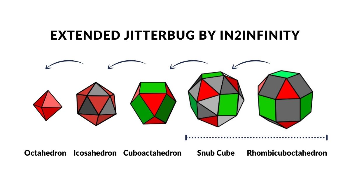
- The Extended Jitterbug — five polyhedra related by continuous geometric transformation — maps the radii of all 81 stable elements
- GQM surpasses the Bohr radius and Van der Waals radius in accuracy for the vast majority of elements
- Apparent randomness in atomic radii — why some noble gases expand and others contract — has a precise geometric explanation
- The model extends Buckminster Fuller's Jitterbug with two additional polyhedra: the Snub Cube and Rhombic-Cuboctahedron
From Atomic Geometry to Geo-Quantum Mechanics
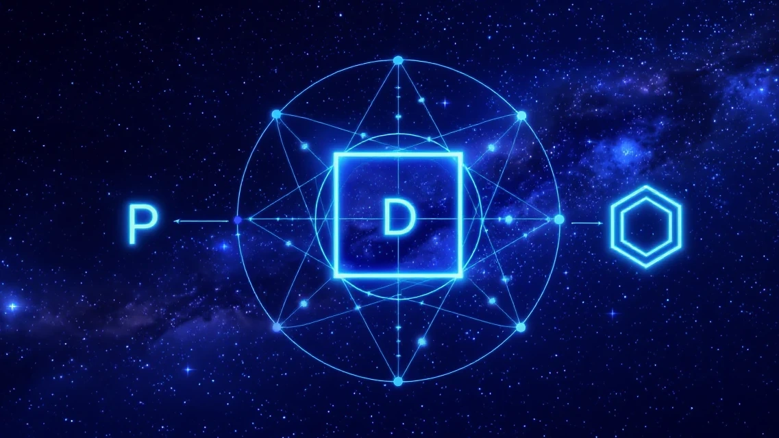
Atomic Geometry establishes the geometric basis of the S, P, D, and F orbitals in the hydrogen atom — showing that each orbital type corresponds to a specific polyhedron. Geo-Quantum Mechanics extends this framework to the entire periodic table.
Where Atomic Geometry focuses on orbital shape, Geo-Quantum Mechanics focuses on orbital size — specifically, on why the radii of atomic shells take the exact values they do as protons and neutrons are added to the nucleus. The answer, it proposes, lies in the geometry of polyhedral transformations: the same geometric operations that relate one polyhedron to another also govern the scaling of atomic radii from one element to the next.
The Cube of Space
Physical space is cubic. The cube is the only regular Platonic solid that fills space completely without gaps — providing the X, Y, and Z axes along which all distances in three-dimensional space are measured.
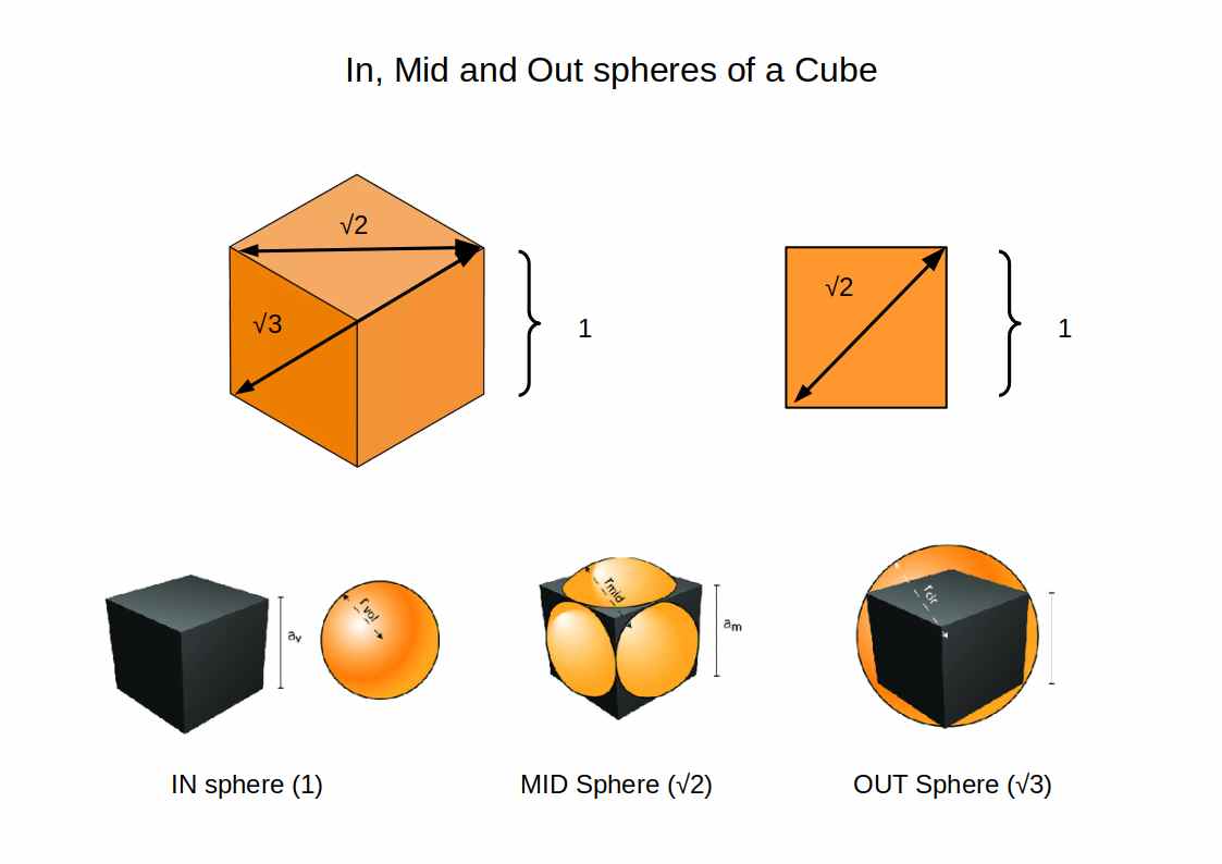
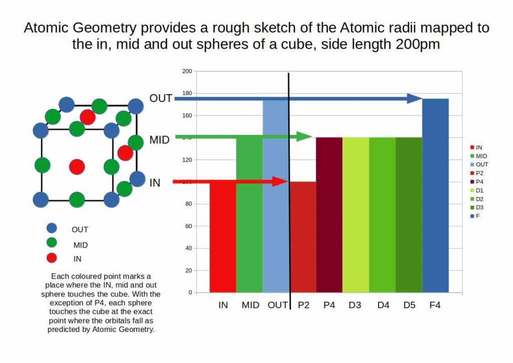
Every polyhedron can be enclosed by three concentric spheres. In Geo-Quantum Mechanics these are called the IN, MID, and OUT spheres:
- IN-sphere: touches the centre of each face
- MID-sphere: touches the midpoint of each edge
- OUT-sphere: passes through each vertex
For a cube with side length 1, the three sphere radii follow the ratio 1:√2:√3 — the same ratios that appear in the electromagnetic constants of Dimensionless Science. These three radii provide the natural scale points at which electrons organise around the nucleus.
Orbital Geometry and the Cube
In Atomic Geometry, each orbital type occupies a specific position within a cube of space: S-orbitals at the centre, P-orbitals along the faces, D-orbitals along the edges, and F-orbitals at the vertices. When the average atomic radius of each orbital block is compared to the IN, MID, and OUT sphere radii of a cube scaled to 2 Å, a direct correspondence emerges.
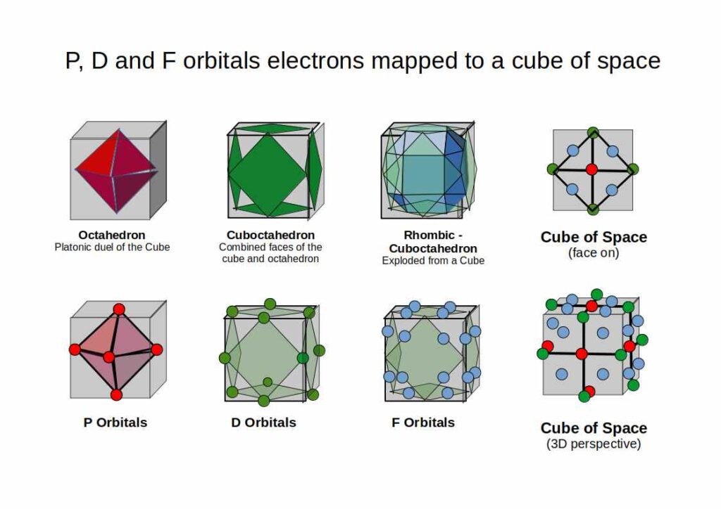
P2-block elements level off at around 100 pm; P4 and D-block elements at around 1.4 Å; the first half of the F-block at around 1.85 Å, contracting to 1.75 Å at the midpoint. These are not arbitrary values — they correspond to the geometric sphere radii of a cube scaled to 2 Å. The geometry determines the scale; polyhedral transformations explain the variation within each block.
Geometric Transformations: The Jitterbug
Geo-Quantum Mechanics is built on two types of geometric transformation: the Jitterbug and Truncation.
Buckminster Fuller discovered that a Cuboctahedron can collapse continuously — when its square faces fold into triangles — into an Icosahedron, and then into an Octahedron. He termed this the Jitterbug and proposed it as an operating principle within atomic structure. Both the Cuboctahedron and the Octahedron correspond to orbital geometries identified in Atomic Geometry.
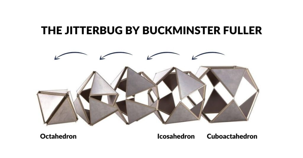
Geo-Quantum Mechanics extends the Jitterbug to five polyhedra with the Cuboctahedron at the centre, forming the Extended Jitterbug. The sphere radii of these five forms, scaled appropriately, account for the atomic radii of all 81 stable elements.
Truncation
The second geometric operation is truncation — removing the corners of a polyhedron by cutting each edge at a fixed ratio. Dividing the edge of a Cube or Octahedron in half produces a Cuboctahedron. Dividing into thirds removes the corners entirely, producing the Truncated Cube or Truncated Octahedron.
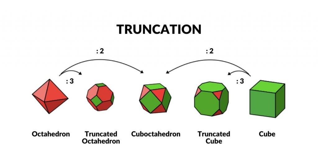
Where the Jitterbug expands the Octahedron outward through the Cuboctahedron, truncation contracts it inward. The two Cuboctahedra produced by each process have side lengths that differ by a factor of two — giving the model its two-scale nested structure.
The Geo-Quantum Blueprint
Combining the Jitterbug, Truncation, and polyhedral compounding produces the Geo-Quantum Blueprint — the complete geometric template used to map atomic radii across the periodic table.
The blueprint is derived from two nested Cube/Octahedron compounds, scaled so that the inner compound has a mid-sphere radius of 50 pm and the outer a mid-sphere radius of 100 pm — values chosen to align the geometry with the experimentally measured radii of the S and P orbital blocks. The compound of the Cube and Octahedron shares the same mid-sphere and jointly defines a Cuboctahedron at its centre. The Octahedron expands through the Extended Jitterbug into the Icosahedron, Snub Cube, and Rhombic-Cuboctahedron. The central Cuboctahedron can also collapse inward into a smaller Octahedron, generating a nested inner compound — scaled so that the inner compound has a mid-sphere radius of 50 pm and the outer compound a mid-sphere radius of 100 pm.
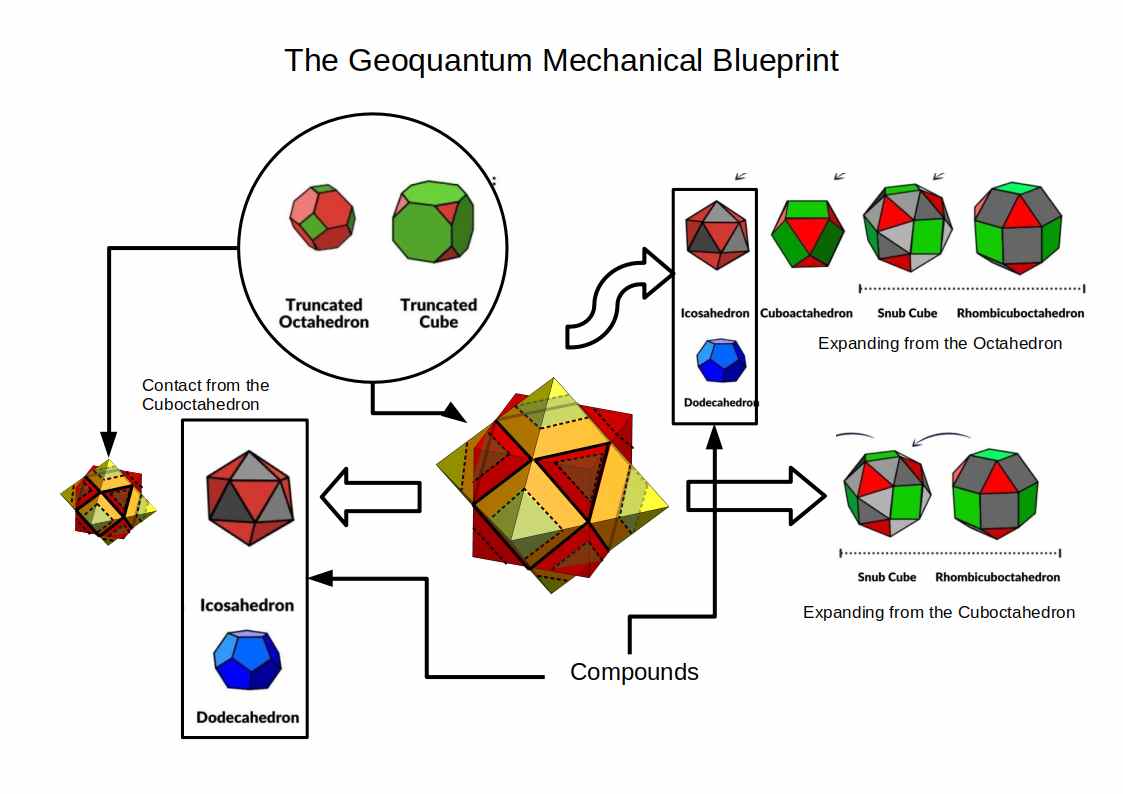
It is the geometry of this nested structure — not the probabilistic behaviour of individual electrons — that Geo-Quantum Mechanics proposes as the organising principle of the electron cloud. The space surrounding the nucleus is geometric, and this geometry holds electrons in stable, quantised shells at specific energy levels.
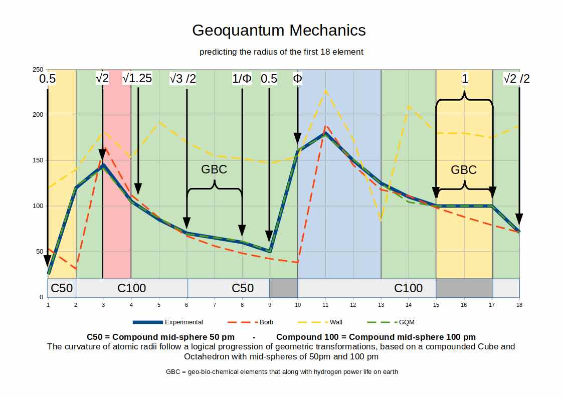
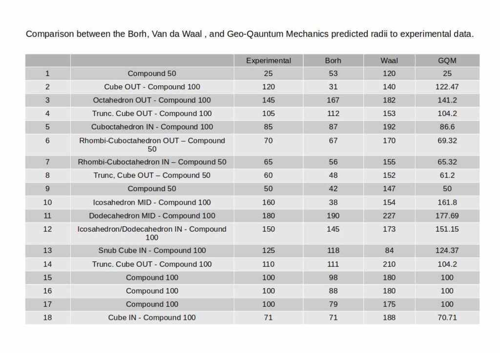
Predicting Atomic Radii
At first glance, atomic radii across the periodic table appear random and unpredictable. Helium (2) is larger than hydrogen (1). Neon (10) is smaller than sodium (11). Argon (18) contracts where potassium (19) expands. Some sequences of elements share almost identical radii; others shift abruptly. No simple rule explains the pattern — and neither the Bohr radius nor the Van der Waals radius comes close to matching the experimental data for most elements.
The Geo-Quantum model explains each variation. Every expansion, contraction, and plateau in the data corresponds to a specific geometric transition within the blueprint: a shift from one polyhedron to another, a move from IN to MID to OUT sphere, or a jump between the two nested compounds. Elements within the d-block (atomic numbers 21–30 and 39–48), for instance, plateau at near-constant radii because their electrons occupy the same OUT-sphere position of the inner octahedral compound — the geometry does not change, so the radius does not change.
Conclusion
Geo-Quantum Mechanics demonstrates that the electron cloud is not a probabilistic fog — it is a geometrically structured space organised by the same polyhedral principles that govern the orbital shapes in Atomic Geometry. By mapping the IN, MID, and OUT sphere radii of a nested polyhedral sequence to the measured atomic radii of all 81 stable elements, the model produces atomic radius predictions that more closely match experimental data than the Bohr model.
The deeper implication is that it is the geometry of the space surrounding the nucleus — not the particle dynamics of individual electrons — that quantises the electron cloud and determines the specific energy levels at which electrons are found. This is the geometric complement to Geo-Nuclear Physics, which applies the same approach to the nucleus itself. Together they form a complete geometric account of the atom from its innermost point to the boundary of the electron cloud — and together they suggest that the periodic table is not a catalogue of chemical accidents but a map of geometric necessity.
FAQ
What is Geo-Quantum Mechanics?
Geo-Quantum Mechanics (GQM) is an extension of Atomic Geometry that examines the electron cloud for all 81 stable elements on the periodic table. By applying the geometry of Platonic and Archimedean solids and their transformations, GQM produces a model of atomic radii that is more accurate than the Bohr radius or Van der Waals radius for the vast majority of elements.
How does it differ from standard quantum mechanics?
Standard quantum mechanics provides highly accurate predictions for the hydrogen atom but struggles with multi-electron atoms. Geo-Quantum Mechanics does not replace quantum mechanics — it provides the geometric framework that explains why atomic radii take the specific values they do across the periodic table, something conventional models cannot account for.
What is the Extended Jitterbug?
The Extended Jitterbug is an expansion of Buckminster Fuller's Jitterbug transformation. Fuller showed that a Cuboctahedron can collapse through an Icosahedron into an Octahedron. Geo-Quantum Mechanics extends this sequence to include two additional forms — the Snub Cube and Rhombic-Cuboctahedron — producing five polyhedra whose sphere radii correspond directly to the measured atomic radii across the periodic table.
What are the IN, MID, and OUT spheres?
Every polyhedron can be inscribed with three concentric spheres: the IN-sphere (touching the centre of each face), the MID-sphere (touching the centre of each edge), and the OUT-sphere (passing through each vertex). In Geo-Quantum Mechanics, these three sphere radii correspond to the radii at which electrons are found in different orbital types — providing a geometric explanation for why atomic radii cluster at specific values.
How does Geo-Quantum Mechanics relate to Geo-Nuclear Physics?
Geo-Quantum Mechanics focuses on the electron cloud — the outer structure of the atom. Geo-Nuclear Physics focuses on the nucleus — the inner structure. Together with Atomic Geometry, they form a complete geometric model of the atom from the nucleus outward to the boundary of the electron cloud. See Geo-Nuclear Physics for the complementary treatment of the nucleus.