DIVIDER FRONT unsmushed

The 2nd set of D-orbitals range from element 39 to 48 on the periodic table. In this article, we examine their geometric structure, and for the first time explain reasons why Technetium (43) should be unstable within the set.

Overview

D-orbital elements are comprised of 5 different types of orbital, each constituted by 2 electrons in opposite (UP and DOWN) spin. 4 of these produce cross shaped lobes, whilst the 5th exhibits a torus shape. In the theory of Atomic Geometry, this structure is based on the Truncated Cube, which defines 2 Rhombic Cuboctahedra at different Scales. This in turn produces the template of the 5D hypercube.

D-orbital Geometry - Part 1

This article is part 2 of a series that explores the geometric structure of the D-orbital Elements Before reading on, we recommend reading the first part that builds on the knowledge explored in this article

KEy Points

  • The 2nd Set of D-orbitals forms a Truncated cube which then trasnistions inot a 5D hypercube the the Icosidodecahedron and Rhombic Cuboctahedron
  • Once the intial element complete half filled orbitals there is contraction of the radius through the Golden ratio
  • This contraction of the orbital radii produces the instability of element 43 within the set.

problems with Quantum theory

Before we continue to examine the nature of the 2nd D-orbital set, let us review some of the key points in the Atomic Geometry Model of the Atom and some of the problems that is solves with present quantum theory. In our examination of the P-orbital elements, we highlighted the fact that many of these elements in each set exhibit the same radius. For example, out of the 2nd P-orbital elements, Phosphorus (15), Sulphur (16), and Chlorine (17), all exhibit an experimentally determined radius of 1Å. In the 3rd P-orbital set, we find exactly the same occurrence. Arsenic (33), Selenium (34), and Bromine (35), all have a radius of 1.15Å. Furthermore, these elements appear in exactly the same place as the P-orbitals form, in groups 15, 16, and 17.

A similar scenario can be found in the other orbital types. For example, except for the initial D-orbital element in the 1st set, the others all express a radius of 1.4Å or 1.35Å. The other 2 D-orbital sets, also have radii that are around the same size. The 1st half of the F-orbital elements all have a radius of 1.85Å, with one element, Gadolinium (64) exhibiting a radius of 1.8Å, before the remaining element of the set all produce a reduced radius of 1.75Å. In terms of the F and D-orbital elements, this uniformity is traditionally explained by F and D block contraction, which suggest this is due to electron shielding, due to the ‘density’ of these orbital types. Yet the mathematical proof of this conjecture is strangely absent from the theory. Additionally, is cannot account for the uniform radii of the P-orbital set, which starts to occur even before and F or D-orbitals form. 

According to the standard model, as the size of the nucleus increases, so the atom should diminish in size. This is often taught as a rule of the periodic table. Yet, upon closer examination, this turns out not to be true. Quantum physics often suggests it can provide an incredibly accurate prediction of the atom. However, when we examine the claim, it is admitted that this is only for ‘hydrogen like’ atoms. Yet even this is not true. For example, the experimentally determined radius of the first element, hydrogen, is 0.25Å. Yet the Bohr Model predicts a radius of 0.53Å, which out by over 100%. Normally, such a discrepancy would require us to re-examine our model, yet instead what we find is that science has chosen to continue to assure the public of its accuracy in prediction, to the extent that if we look up the radius of the hydrogen atom, rather than providing us with the experimentally determined radius, we are presented with the theoretical prediction. Only by digging deeper into the datasets, are we able to uncover this truth.

Let us reconsider this information in the light of geometry. From a radius of 0.25Å for Hydrogen (1), the 1st P-orbital set falls in size until Fluorine (9) which has a radius of 0.5Å. In the 2nd P-orbitals, the radius settles at 1Å. A clear doubling sequence. After this, the 3rd P-orbitals, we find a similar phenomenon with at a radius of 1.15Å. The difference between this 2nd and 3rd set is actually described by the difference between the out and mid-sphere of a Rhombic Dodecahedron, which forms the template of the 4D hypercube. The 4th P-orbitals, which forms the last complete set of the stable elements of this type, exhibit a radius of 1.45Å and 1.4Å, which is around √2, and also happens to be roughly the size of D-orbital elements. Finally, the F-orbitals fall in size to 1.75Å, which is close to √3. Note that the ratios of 1, √2, and √3 are found as the in, mid, and out-sphere of a cube with a side length of 2.

Without a great deal of tweaking, the Atomic Geometry model already provides a very good approximation of the structure of the electron cloud. However, we can even go one step further, by closely examining the geometric transformation of each element, which can explain in intricate detail the subtle changes in atomic radius, as well as the reason for the conductive and magnetic properties of various elements, which is explained in our post on the geometric nature of the Brillouin Zones.

Before we move on, let us consider one other major contradiction in the present theories of quantum mechanics. At the forefront of this interpretation of the atom are the Schrödinger equations. These are often thought of as being wave equations, which are supposed to predict the behaviour of quantum particle interactions, or more accurately the probability of finding an electron at a given location. However, on closer examination, it turns out that these are not wave calculations as is commonly taught. Instead, they are more akin to heat equations, which predict the flow from one state to the next. However, as the atom is quantised into discrete bands or shell, this flow cannot be considered as a continuous motion. This is explained in detail in this video, by the Science Asylum.

Notice that at the start of the video the presenter explains that electrons are not really particles, they are actually tiny waves that give the ‘illusion’ of being tiny particles. The wave nature of electrons was first proposed by Louis de Broglie in 1924, and were experimentally confirmed by the Davisson-Germer experiment. It was this idea of Louis de Broglie that lead Erwin Schrödinger to develop the mathematical formula of his equations. These were later adapted to include the quantised spin nature of the electron, which can only exhibit 1 of 2 states, UP or DOWN.

However, the Schrödinger equations do not express waves. Instead, they show the transformation of the electron cloud from one state to the next, and this is where we find the next contradiction emerging. On the one hand, the transfer of heat or the bouncing of a spring (wave) are continuous, not discrete values as in found in the nature of the quantum world. This means there are only certain values that an electron can take. What the Schrödinger equations are depicting is a flow between probabilistic states. Now here comes the stinger. Sometimes you will hear physicists state that the electron has a probability of being in any location, as in the video above. Other times you will here is confirmed that it can only appear at certain quantised states, or energy levels, which in quantum mechanics determines how far from the nucleus the electron can be found. So which is it?

At it core, the problem arises from the insistence of quantum mechanics to consider the electron, and even light for that matter, as a particle. This notion of wave-particle duality stems from the inability of science to resolve the Ultraviolet catastrophe and Photoelectric effect without reintroducing the particle nature of light. However, the mistake, whilst imbued in heavy mathematics, is quite easy to unravel. Rather than basing the calculations on resonance, which is how different waves interact, it was decided to employ the harmonic series. This is explained in greater detail in our wave only solution to these problems.

For most scientists, these solutions are highly controversial, as it begins to undo over 120 years of scientific thinking, and reintroduces the theory of the Aether, from the perspective of 4D geometry. However, once the wave only solutions are adopted, what emerges is a logical and consistent theory, which does away with all notions such as wave-particle duality, probability theory, and quantum entanglement. This explains the notion of quantised spin values as the rotation of 4D and higher dimensional polytopes, which form the boundaries produced by the atomic structure. The energy density of the vacuum (Aether) is what produces the mass of the atomic nucleus, which in turn produces the electron field.

What makes this theory particularly unpopular with popular science, it that it has expended vast amounts of energy discrediting the notion of the Aether, something that was a common belief in the science predating the particle notion of light. Yet, this model provides a much more accurate description of the atom than any other that exists today.

It is an easily demonstrated fact that whenever humanity loses touch with the geometric nature of reality, as is the case after the destruction of Alexandria in the times of the ancient Greeks, or the collapse of the Islamic Golden age, so its progress is largely hindered. The age of the Renaissance begins with the rediscovery of the Platonic and Archimedean solids, which lead to the revelations of Newton that changed the landscape of scientific thinking. Similarly, in our modern age, the invention of technology, such as the laser, was suggested by the pioneers of particle physics to be an impossibility. Today, the laser has transformed global communications, and finds application throughout the modern world. Subsequently, particle theory had to be adapted to explain this phenomenon. Yet at no point did anyone try to re-evaluate the mathematical procedures that have produced such a contradictory system, as proposed by the quantum mechanical model that stands today.

The theory of Atomic Geometry therefore suggest that the Schrödinger equations are really depicting the transformation of one solid to another. This is what forms the quantised states depicted by quantum mechanics. With each progressive atom on the periodic table, the geometry of the Nucleus and electron cloud changes shape, which produces the variation in atomic radii, and quantises the electron cloud into discrete bands, due to the nature of the in, mid, and out-sphere of each solid.

Before reading on, we suggest that the reader examine some of the posts linked above, in order to gain a wider appreciation of these inconsistencies, and to deepen their understanding of the principles of geometry that will be discussed in the article. Once a notion of these geometric principles are comprehended, we guarantee you will quickly be able to see how Atomic Geometry resolves many of the issues imbued in our current understanding of the universe, and the importance of these resolutions that we are proposing.


Geometric Principles

The theory of Atomic geometry is predicated on a series of geometric principles. Firstly, any 3D solid produces an out, mid and in sphere. For example, a cube, has an in-sphere that touches the middle of each face, whereas the mid-sphere divides the midpoint of each side. Finally, the out-sphere touches each of its corners. This simple concept can be used to explain the quantisation of the electron cloud. In other words, the reason why the electron energy is quantised into bands it due to this geometric nature. Therefore, the probability transformations predicted by the Schrödinger equations are due to this fact. It is the geometric nature of ‘space’ that produces the quantisation of reality. 

The second Geometric Principle that govern this quantisation is found in the nature of the Jitterbug Construction. This was originally popularised by Buckminster Fuller, who in fact suggest that it can be used to model the compositions of various substances. However, in his expression of this structure, he only included 3 forms. The Octahedron, Icosahedron and Cuboctahedron. The theory of Atomic Geometry adds another 2 solids to the construct, the Snub Cube and Rhombic Cuboctahedron. We call this the Extended Jitterbug.

These series of solids can be transformed from one to the next by opening the sides of the Octahedron to form 2 triangles, which produces the Icosahedron, As the newly formed gaps expand beyond 2 triangles it forms the square sides of the Cuboctahedron. This structure can also be expanded into the Snub Cube and Rhombic Cuboctahedron through the same process. In the above diagram, you can see that various geometric constants are defined. The Octahedron incorporates the ratio 1:√2, whilst in the Rhombic Cuboctahedron are the end of the sequence add a 1 to √2 to produce the Silver Ratio (√2±1) found in the Octagon. The Icosahedron contains a pentagonal midsection, which contains the Golden Ratio (Φ), whereas the Snub Cube, (2nd from last), expresses the Tribonacci constant, (similar to the Golden Ratio but using 3 terms). At the centre, the Cuboctahedron is the only sold whose side length is the same as its radius, which makes it the perfect form to nest 13 spheres in space, often termed hexagonal close-packing.

The form can also be inverted, which is indicative of a 4D polytope, which we ascribe to the quantised nature of electron spin, which exhibits an UP or DOWN quantised state. Whilst present quantum theory does have a similar analogy to this, called spinors, this sees streams attached to the outside of the object, rather than being intrinsic to itself, which is the very definition of ‘intrinsic angular momentum‘, aka, spin. However, a more accurate description is found in the rotation of the 4D hypercube on its w-axis (time axis), which also produces quantised ½ integer spin values, which we explain in our article on the 4D Electron Cloud.

Electron spin described by different geometric models. Spinors (left) used in traditional quantum theory, The inverted Jitterbug (centre), and 4D tesseract found in the theory of aomic Geometry.

The other two geometric principles that produce different forms are truncations and explosions. An example of an exploded solid is the Rhombic Cuboctahedron. When the sides of a Cube or Octahedron are moved away from the centre, new spaces appear that can be filled with more square faces. Therefore, its 8 triangular faces are derived from the Octahedron, whereas 6 of its square faces a produced from the Cube. This geometric transformation is discussed in great detail in our examination of the 1st D-orbital set.

The Octahedron and Cube can be exploded to form the Rhombic Cuboctahedron

Truncation is the process of removing the corners of a solid at either the halfway or one third of each side length and removing the corners. The Cuboctahedron is also an example of an Octahedron or Cube, that has been truncated at its halfway point. Truncation is most commonly recognised in the formation of 7 of the 13 Archimedean solids.

Truncation of a solid’s sides at the midway and one third produces a set of 7 Archimedean Solids (Truncated Tetrahedron not shown)

Notice that the Cube and Octahedron are found at the end of the top rows, and Dodecahedron and Icosahedron in the bottom row. Each have corner points that are of the same number as the others faces. These are termed ‘Duals’, which is another geometric principle of geometry. An Octahedron can be placed inside a Cube, so that is corners define the centre of its faces, and vice versa. The nesting of solids is another geometric principle, although not all nest pairs are formed of duels. For example, a Cube can be nested inside a Dodecahedron. In this case, it can be orientated in different locations, which we will discuss in more detail shortly.

The final geometric principle we need to know about is that of compounds. A pair of solids can be positioned in such a way as so that the mid-spheres of each is aligned. A good example of this is the Cube and Octahedron. Once compounded, the corner caps can be removed to form a Cuboctahedron, sometimes termed the ‘Hull’ of the compound. By connecting the corner points of each of these compound solids, a Rhombic Cuboctahedron is formed. The Rhombic Dodecahedron produces the template for the 4D hypercube, (tesseract), which is pictured next to the inverted jitterbug in the previously.

These are the foundational geometric principles that form the basis of the Atomic Geometry model of the atom. These produce logical geometric transformations that, just like the Schrödinger Equations, show how one solid (orbital shape) can transform into the next. However, instead of being based on probability density, the concepts produced in the Atomic Geometric model are purely spacial. Whilst the atom is elusive, difficult to measure, and define, (due to its 4D and higher dimensional nature), we can produce an exact description of each element, its size, and the reasons for it particular properties through this set of 7 geometric principles.

  1. In, Mid and Out-spheres
  2. Nesting
  3. Duels
  4. Compounds
  5. Truncation
  6. Explosion
  7. The Jitterbug

Through this, we can build a geometric blueprint that explains how space can evolve from the 5 Platonic Solids into other forms, including 4D, 5D and 6D polytopes, and beyond.

4D, 5d, & 6D Hypercube

Now that we have clarified the geometric principles of Atomic Geometry, we can now explore how these forms evolve and interact to produce the foundations of the atomic structure, for the D-orbital elements. For the S-orbitals and P-orbitals these are express as a Sphere and Octahedron respectively, that are explored in greater detail in our articles on the subject. The 1st D-orbital are explained by the 4D Rhombic Cuboctahedral model, covered in the 1st part of this article. When constructed from the explosion of a cube with a side length of 1, the Rhombic Cuboctahedron produces an out-sphere of 1.4Å. When this collapses through the Jitterbug Transformation into the Snub Cube, it creates a smaller out-sphere of 1.35Å, which produces the main 2 types of radii found in the 1st D-orbitals set. This provides a simple overview, which is expanded upon in the 1st part of this article.

Discover the Atomic Geometry of the 1st D-orbital elements

In our exploration of the 1st D-orbital elements, we explained how the combination of the Octahedron and Cube produces the Rhombic Dodecahedron, which is the template for the 4D hypercube, or Tesseract. At the end of the article, we also suggest that the Dodecahedron is actually the template for the 5D hypercube, something that is not presently recognised in the field of modern geometry. This observation comes about as a Cube can be nested inside a Dodecahedron in 5 distinct orientations. When completed, each face exhibits a penagram, or 5-pointed star, formed by the side of each cube.

The second observation is that the Dodecahedron can be nested around the Cube in two distinct orientations. This is similar to the notion of the Tetrahedron, which can be combined with another tetrahedron to form a star-tetrahedron that, when nested inside the Cube, defines its 8 corners. Similarly, 8 of the Dodecahedrons 20 corners also defines the corners of the Cube. The remaining 12 corners fall into 6 pairs, orientated above the face of each cube.

Finally, The cube itself can be rotated through four 90° orientations, on its north-south axis. This brings the total number of Cube up to 40, which is the number of Cubic faces that form a 5D hypercube. Each of the 4 rotations of the Cube can also be envisioned as a single Tesseract Cell, of which 10 make up the faces of the 5D cube.

Corners
Cubic Faces
Tesseract Faces
32
40
10

The 5D Cube also has 32 corners (25). This number is equal to the combined corners of the dodecahedron and Icosahedron Duals. When compounded, the corners of these solids can be connected to form the Rhombic Triacontahedron. Similar to the Rhombic Dodecahedron, which is the template for the 4D hypercube, the Triacontahedron is the template for the 6D hypercube. Thus, our proposal that the dodecahedron forms the template for the 5D cube fits into a simple geometric sequence of that begins with a 3D cube, which is compound with the octahedron to form the 4D cube, which is then nested in the Dodecahedron to form the 5D cube, which is finally compounded with the Icosahedron to form the template of the 6D Cube.

Finally, we should point out that a 4D Cube often depicted as one cube nested inside another. This is analogous to a 3D shadow projection, where the size of one cube is reduced, as if the light source is moved slight further away for that particular part of the Tesseract, (as seen above). A similar shadow projection can also be applied to the 5D cube to produce an image of 3 nested Cube, which we will discuss in more detail shortly. Similarly, the 6D cube can be constructed from a nested set of 4 Cubes. However, we suggest that the 5D cube can also be depicted by replacing the 2 Cube with Rhombic Dodecahedra, whereby the middle cube of the three becomes shared between the 2 Tesseracts. Similarly, the Cubes can be replaced by 2 Rhombic Triacontahedra, to represent the shadow projection of the 6D Cube.

This produces a new simplified expression of higher dimensional cubes that is presently missing from our understanding of geometry. Armed with this new knowledge, we can now proceed to decode the higher dimensional geometric nature of the atom, and for the first time reveal the answer to some of the most perplexing aspects of the electron configuration that has, until today, remained a complete mystery to the world of science.

Atomic Geometry model of the 2nd D-orbital elements.

In the theory of Atomic Geometry, the first D-orbital sets are modelled by a Cube with a side of 1, that explodes to form the Rhombic Cuboctahedron. A second Cube with a side of √2 also nests inside this structure, with its corners centred on the triangular faces of the Rhombic Cuboctahedron. This larger cube can be truncated to produce a Cuboctahedron with a side of 1. Similar to the Rhombic Dodecahedron, this nested structure also produces a model of a 4D hypercube. In fact, in our article that explores the 1st D-orbital set, the wire frame of the Rhombic Dodecahedron is shown to produce the shadow projection of this geometric construct when viewed from above.

The second D-orbital set builds upon the foundation of this structure. Instead of forming a Rhombic Cuboctahedron, the initial orbitals are instead represented by the Truncated Cube. Both of these forms exhibit an Octagon. In the Rhombic Cuboctahedron, this appears as the mid-section, which can be rotated in quantised steps of 8. In the Truncated Cube, the Octagon appears on each of its six sides that are derived from the Cube. The Octagon contains the Silver Ratio (√2±1), which is similar to the Golden Ratio, which is most commonly express within a pentagon.

Let us next examine the geometric relationship between the Rhombic Cuboctahedral Model of the 1st D-orbital set, and the Truncated Cube that constitutes the 2nd D-orbitals. By removing the square faces of the Rhombic Cuboctahedron, we can reveal the Cube that sits at the centre of its structure. On each of its corners, there are 8 sets of tetrahedral solids with sides in ratio of 1:√2. This form is called the Anti-Truncated Cube. A similar process when applied to the Truncated Cube generated the Hyper-Truncated Cube. At the centre of this structure is a form that is similar to the Truncated Octahedron, however, the hexagonal faces are also in a ratio 1:√2.

The Rhombic Cuboctahedron can be divided into 3 sections, with a central octagonal prism which can be rotated in 45° quantised steps. In the 1st D-orbital Model, this is used to explain the 5th Torus orbital in the set of 5, as the midsection can be rotated without moving the top and bottom sections. In the Truncated cube, these top and bottom sections are inverted, so that the square face now touch those of the Cube at the centre. This produces a central column, which lies at the centre of a torus field. Notice that this produces 4 spaces adjacent to each face of the cube. When viewed from above, each set of 4 appears in a cross shaped orientation, which is indicative of the 4 D-orbital lobes.

The Truncated Cube can also be defined by 16 interlocking squares that form the ‘Non-convex Great Rhombic Cuboctahedron’. Upon close examination of this form, we can see that it defines 2 Rhombic Cuboctahedra, nested at different scales. If the larger has a side of 1, then the smaller will exhibit a side of √0.5, or √2÷2. Notice that when the square sides, those that originate from the exploded cube that generates the form, are projected outwards, each will fall inside the 8-pointed star formed at the centre of each face of the Non-convex polyhedron. This relationship expresses the Sliver Ratio, as √0.5±½.

In this way, the Truncated Cube is able to orientate 2 Rhombic Cuboctahedra. Whereas a single Rhombic Cuboctahedron produces a model of 4D Cubic Space, when two are combined it creates the template for 5D cubic space, which is orientated through the Silver Ratio.

The non-convex great Rhombic Cuboctahedron consists of 16 square planes. 6 of these fall into the horizontal and vertical and orientations, whilst the other 10 fall across the diagonals of the structure. If we extract the 6 vehicle plains, they divide a cube of space into 27 small parts (3³).

However, as the corners are removed from the Truncated Cube, this number is reduced to 19. A complete D-orbital set is formed of 5 orbital types, 4 of which are ‘cross shape’ in nature. The 5th Orbital is formed of a torus with 3 lobes in the north and south orientation. If we count the torus shape as a single lobe, there are 18+1=19 in total, which is the same as the number of cubic spaces produced by the Non-convex form.

However, each space in not a Uniform Cube, due to the nature of the octagonal faces of the Truncated Cube. Only those that exists in the central plains are uniform, which is where the torus D-orbital and one of the ‘rotated’ cross D-orbitals are located. In Atomic Geometry, we differentiate between these two types as the 2 Torus orbitals and 3 Cubic orbitals, as the latter define the midpoints of the side of a Cube. The Torus orbital pair fall in the same orientation as the P-orbital sets.

When we deconstruct the Non-convex Great Rhombic Cuboctahedron, we find that the 2 nested Rhombic Cuboctahedra are able to produces a geometric structure that can be mapped to the 2nd D-orbital set.

A Rhombic Dodecahedron is composed of a compound of a Cube and Octahedron. In the structure of the electron cloud, the 3rd P-orbital set form over a completed set of D-orbitals. Therefore, in Atomic Geometry this set is represented by this compound, which forms the template for 4D hypercubic space. This is why the radii settle at 1.154Å, rather than continuing to double in size. The previous P-orbitals have a radius that settle at 1Å, so we find that the difference between the 2 sets is found as the mid and out-sphere of the Rhombic Dodecahedron.

In Atomic Geometry, the 1st D-orbital set is represented as a Rhombic Cuboctahedron, which can be created by truncating a Rhombic Dodecahedron. When the second orbital set forms, it produces a second Rhombic Cuboctahedron, as pictured in the image above, whose size and spacing is defined by the Non-convex Great Rhombic Cuboctahedron, which is generated by the Truncated Cube. The Rhombic Dodecahedron can be placed around the smaller Rhombic Cuboctahedron, so that its outmost corners, (those created by the Octahedron), touch the centre face of the larger Rhombic Cuboctahedron. The combination of the Truncated Cube and Rhombic Dodecahedron therefore produce the relationship between the 2 different sized Rhombic Cuboctahedron, which, in our view, forms a template 5D Hypercubic space.

Play Video

Da Vinci School Online course

Atomic geometry

Build a geometric model of the atom

The most fun, creative and tactile exploration of the atom, based on Schrödinger Equations, giving you a solid foundation for physics and chemistry.

Transition from the 1st to the 2nd D-orbital set

After the 1st Orbitals complete in the 3rd shell of the atom, (elements 21-30), a 3rd set of P-orbitals, (element 31-36), start to form in the 4th shell. This is not immediately obvious by examining the periodic table, as the D-orbital sets are portrayed in terms of proton count, rather than electron configuration. As more protons appear in the atomic nucleus, so the different types of elements form. After Potassium (19) and Calcium (20) form in the 4th shell, the 1st D-orbitals go on to fill in the 3rd shell below. Therefore, D-orbitals tend to exhibit a set of S-orbital electrons in the shell above, although there are exceptions that we shall examine in more detail shortly. Once complete, the next set of 6 P-orbital elements (31-36) form in the 4th shell. Then the pattern repeats with 2 S-orbital elements, (37 and 38) forming in the 5th shell, before the 2nd D-orbital set begins to complete, again in the shell below, which is the 4th shell.


After the 1st D-orbitals complete with a radius of 1.35Å, the P-orbitals that start to form exhibit a progressively smaller radius, until the 3rd element of the set. At this point Arsenic (33), Selenium (34), and Bromine (35), all exhibit the same radius of 1.154Å.

This fact contradicts the standard model, that suggest the subsequent atoms should all exhibit a progressively smaller radius, as more protons are added to the nucleus. The theory of Atomic Geometry offers a very simple solution, as pointed out previously. The radii from the 2nd and 3rd P-orbitals is simply explained as the difference between the out and mid-sphere of the Cuboctahedron, or more accurately, the Rhombic Dodecahedron. Furthermore, as the Octahedron is contained within the structure of the Rhombic Dodecahedron, it too can be produce by truncating the corners it’s corners.

As the 3rd P-orbitals form after the 1st D-orbital set, so they produce a different geometry, compare the those P-orbitals that precede it. This is the reason why the only exhibit of radius of 1.154Å, rather than a radius of 2Å, which would be the case if the doubling of radii were followed, as with the previous P-orbital types.

S-orbitals elements generally exhibit a much larger radius than the other orbital types. Rubidium (37), for example, has a radius of 2.35Å, which is more than double that of the preceding P-orbitals. This is followed by Strontium (38) with a radius of 2Å.

The Cuboctahedron with a side of 1.154Å has a mid-sphere of 1Å, which defines the radius of the 2nd and 3rd P-orbitals. The dual of the Cuboctahedron is the Rhombic Dodecahedron. This is composed of a compound of the Octahedron and Cube. The Octahedron has a side double that of the Cuboctahedron, of around 2.3Å, or more accurately, 4÷√3, which produces an Out-sphere of 1.63Å. The Cube has the same side length of 1.63Å, and out-sphere of √2, or 1.41Å. Also, the Midsphere of the Rhombic Dodecahedron is 1.33Å. Together, these 3 radii, 1.63, 1.41, and 1.33, provide an extremely close match to the 3 types of radius found in the 1st D-orbital set.

The Octahedron can be transformed into a Cuboctahedron, through the Jitterbug transformation. This produces a larger out-sphere with a radius of 2.3Å, which roughly the size of Rubidium (37), which appears after the 3rd P-orbital (elements 31-36) are formed. This also has an in-sphere of 2Å, which is the radius of Strontium (38), that completes this S-orbital set.

However, we also find that the Icosahedron which forms between the transition of the Octahedron to the Cuboctahedron in the Jitterbug, has a radius of 2.18Å for its out-sphere, and 1.86Å, which defines the radii of the preceding S-orbitals, Potassium (19), and Calcium (20), which form just prior to the 1st D-orbitals. Thus, this simple geometric model maps all radii from element 19 through to 38. This is explained in greater detail in the 1st part of this article.

Just as the Octahedron and Cube can be compounded, the same can be said of the Icosahedron and dodecahedron pair. As before, this is achieved through the unification of the mid-spheres of each solid, which is a radius of 1.86Å. Not only is this the radius of Calcium (20), but it also defines the size of the first D-orbital Element, Yttrium (39), and the first 6 elements of the F-orbital set, which appear in the same shell. Note that the last 7 F-orbitals also exhibit a radius produces by the In-sphere of the Icosahedron.

When compounded, the Dodecahedron will exhibit an out-sphere of radius 2Å, which is the same value as the Mid-sphere of the Cuboctahedron, and Strontium (38). The mid and in-spheres of the dodecahedron produces 2 other radii, of 1.86Å and 1.59Å, which produces a close match to that of the 1st and 2nd elements in the 2nd D-orbital set, Yttrium (39), and Niobium (40). Thus, in this geometric construct we have defined the radii of all the elements from Phosphorus (15) with a radius of 1Å in the 2nd P-orbital set, right the way through Zirconium (40), as well as all but 1 of the F-orbitals elements

Atomic Radii : Red = P-orbitals, Green = D-orbitals, Blue = F=orbitals

As the Rhombic Dodecahedron is produced from the compound of an Octahedron and Cube, which is formed by the combination of the 1st D-orbital set and 3rd P-orbitals in the shell below, there is another type of geometric transformation that can occur. The Cube that nests around the Cuboctahedron can also be placed inside a Dodecahedron. These will both share the same sized out-sphere, with a radius of 2Å. The mid-sphere of the Cube will be 1.154Å, which is the average radii for the 3rd P-orbital set. The Mid-sphere of the Dodecahedron will be slightly larger, with a radius of 1.32Å. When compounded with an Icosahedron, they form the Rhombic Triacontahedron, which forms the template for 6D hypercubic space. This produces a slightly larger out-sphere of 1.55Å, which is the radius of the 2nd element, Zirconium (40), in the 2nd D-orbital set.

The Rhombic Triacontahedron has a mid-sphere of 1.47Å, which is the radius of the next 2 elements Niobium (41), and Molybdenum (42). This is only fractionally larger than the out-sphere of the Truncated Cube that is derived from a Cube with a side length of 2.

In order to grasp this geometric nature in more detail, we need to examine the order in which the various orbital types begin to construct the geometry of these D-orbital Elements. The preceding S-orbitals appear in the 5th shell above the 2nd D-orbital set. These radii (2.3Å and 2Å) all appear in the Jitterbug transformation, shown in the bottom row above.

When the first D-orbital element forms, the radius contracts to 1.85Å, found in the Mid-sphere of the Icosahedron and Dodecahedron compound. This orbital is formed from the 1st of the torus orbital types. With the next element, Zirconium (40), the torus orbital set completes. Thus, the radius contracts, falling into the smaller Icosahedron, found in the top row above.

After this, the pattern should repeat with the next orbital creating a radius of 1.32Å, which is the mid-sphere of the Dodecahedron. However, as the torus is already complete, the Cubic D-orbitals begins to form. This changes the structure of the atom, producing the Truncated Cube. At this point, we find that instead of a single D-orbital being added to the set, Niobium (41) transforms one of its S-orbital electrons into an additional D-orbital electron, which creates an anomaly in its orbital configuration that we will discuss in more detail shorty. This sustains the Truncated Cube, by producing 4 orbital lobes above the torus ring, and 4 below. The next element, Molybdenum (42), then completes the D-orbital set. Notice that the 1st elements comprised of the Torus Orbitals are formed from the Icosahedron, which has a rotatable mid-section, where the torus ring appears, which when the 2 Cube D-orbitals from in the subsequent element transforms the geometry into a Truncated Cube.

In order for us to really appreciate the accuracy of prediction produce by the theory of Atomic Geometry, we can compare it to the data provided by experimental measurement, and to the predictions based on the Bohr Radius. The experimental dataset is suggested to be accurate to within a margin of ±5Å. The Bohr radius is based on the standard model. As we can see, more often than not, the results fall outside the experimentally determined margin of error. The Atomic Geometry Model on the other hand consistently falls within these limits. Note that the reason for the error produced by the standard model is normally attributed to D-block contraction. Yet on closer examination, the mathematical nature that can support such an idea is strangely absent. If it did exist, then science would have surly applied it to the mathematical calculations, in order to improve the quantum physical model. Furthermore, the theory of contraction cannot account for the uniformity of the elements in the P-orbital set, which presently hold not clearly defined explaination.

Critics of the theory of Atomic Geometry might assume that we have selected the values of the solids in order to fit the experimentally determined values. However, this is not the case. The model simply follows the geometric principles that we have defined at the start of this article. Furthermore, we can also offer a detailed explanation that reveals the reason for many of the intricate details of the electron cloud, which cannot be explained by any other model.

As we have shown, the first 2 D-orbital elements are found in the out and mid-sphere of the dodecahedron, which we beleive forms the Blueprint of 5D Hypercubic space. The elements in the preceding shell, complete the template of 4D hypercubic space, through the structure of the Rhombic Dodecahedron. As each D-orbital set completes, it advances through higher dimensional cubic space.  A shadow projection of a 4D hypercube can be considered as 2 cubes that nest inside each other. This is explained by the 1st D-orbital model, which is formed of 2 cubes, one with a side of 1, and a second with side √2. The 2nd D-orbital set start to construct a 3rd Cube, which is indicative of the shadow projection of a 5D hypercube, formed of 3 nested cubes, which can also be considered are 2 nested tesseracts, where the middle cube is shared between the set.

4D Hypercube

5D Hypercube

As the nature of the 5D hypercube is expressed through the Dodecahedron, we can see that the idea that the first 2 D-orbital sets should be represented by the out and mid-sphere of this form is not just an arbitrary association. Instead, it follows the blueprint defined by the principles of geometry, and its transformation into higher dimensional space.

Element 43

As noted previously, the electron configuration of the D-orbital elements is generally composed of a pair of S-orbital electrons that appear in the shell above the D-orbital electrons. This is described by the Aufbau Principle, which we explain in greater detail in our 1st article on the D-orbital elements. However, there are exceptions. In the 1st D-orbital set, Chromium (24) and Copper (29) only exhibit a single S-orbital in the outermost shell. In the 2nd set of D-orbital elements, the number of anomalies increases dramatically, to the extent that more elements break the Aufbau principle than follow it.

This begins with Niobium (41), which contains 4 D-orbital electrons, and only a single S-orbital electron in its outermost shell. The pattern continues for the next element, Molybdenum (42), after which Technetium appears, which is strangely radioactive. Then another 2 element form with only 1 S-orbital, after which Palladium (46) prematurely completes a full set of 10 D-orbital electrons, removing all S-orbitals from its outer shell. The final 2 elements see the return of the S-orbital electron until the full set of D-orbitals complete.

Up electrons
Element
D-orbital
S-orbital
Radius
Yttrium (39)
1
2
1.8
Zirconium (40)
2
2
1.55
Niobium (41)
4
1
1.45
Molybdenum (42)
5
1
1.45
Technetium (43)
-
-
1.35
Down electrons
Element
D-orbital
S-orbital
Radius
Ruthenium (44)
7
1
1.3
Rhodium (45)
8
1
1.35
Palladium (46)
10
-
1.4
Silver (47)
10
1
1.6
Cadmium (48)
10
2
1.55
Previously, we explained that the reason why Niobium (41) and Molybdenum only exhibit a single S-orbital electron is due to the fact that these elements from the geometry of a Truncated Cube. This requires Niobium (41) to form with 4 D-orbital electrons, in order to maintain a balanced structure with the 2 torus D-orbitals shapes that form with the previous 2 elements. The D-orbitals then complete with Molybdenum (42).
 

The next Element, Technetium (43), returns the S-orbital electron to its outer shell. Yet this element is strangely radioactive, which means that over time it will decay into either Molybdenum (42), or Niobium (41), when synthesized in a laboratory.  The reasons for this are geometric in nature. Firstly, let us consider the structure of the electron cloud as a whole.  There are 3 stable D-orbital sets. What we notice is the element 43 falls at the halfway point in the construction of the D-orbitals, sets. If we consider each set to form a cubic formation, then there is one complete cube ‘above’, and one ‘below’. When nested in a set, this forms the shadow projection of a 5D hypercube. When a 4D cube is rotated on its w-axis (time axis), the cubes swap places. The 5D cube is formed of 4D tesseract faces, which is has a shadow projection of 3 Nested Cubes. In the shadow projection of the 5D Cube, the middle Cube becomes shared between the outer and inner projection of the tesseract cell. This produces an instability at the halfway point of the middle Cube, whereby it remains at the centre as the other two rotate around each other. In the D-orbital set, we find a similar process at work which prevents element 43 from being stable.


We can also explain the reason for the instability of element 43 from the perspective of geometric transformation. As noted previously, Molybdenum  (42) exhibits a full set of D-orbitals, but with only 1 S-orbital electron in its outermost shell. This element has the geometry of the Truncated Cube, with a side of 0.828 (√8-2), and an out-sphere of 1.47Å.

When Technetium (43) returns its S-orbital to its outmost shell, the atom develops a north-south pole. This pushes through each face of the Truncated Cube, increasing the size of the Octahedron (or Rhombic Dodecahedron) that is formed by the preceding P-orbital set. This in turn collapsed the cubic form of the Truncated cube, and transforms it into an Icosidodecahedron, to produce a slightly smaller out-sphere of 1.34Å, which is roughly the same as that of Technetium (43) when synthesized in a laboratory.

The Truncated Cube has 24 corners, which when subtracted from 42, the number of protons found in Molybdenum, leaves 18. When we examine our model of the 2nd D-orbital set, we find there are 18 locations filled by each of the D-orbital lobes. This is also the number of corners found on the Tetrakis Cuboctahedron, which has slightly extruded centre points on the square faces of the Cuboctahedron.

When an extra proton gets added to the nucleus to create Technetium, this geometry shifts dramatically, as the Icosidodecahedron now has 30 corners, instead of 24 that is found in the Truncated Cube. The Tetrakis Cuboctahedron transforms into its Dual, the Truncated Rhombic Dodecahedron, which also has 30 corners. This then compounds with the Cuboctahedron which is able to nest 13 spheres in space, termed hexagonal close packing (HCP), bringing the total number of corners up to 42+1 at the centre. This collapses the Truncated Cube, which now becomes a Rhombic Cuboctahedron, which is defined by 24 of the corners found in the Truncated Rhombic Dodecahedron.

What we can see is that as the elements progress from 42, which exhibits a full complement of half filled D-orbital electrons, up to the unstable Technetium (43), there is a shift in dimensionality, from the Truncated Cube and Tetrakis Cuboctahedron, to the Truncated Rhombic Dodecahedron and Cuboctahedron compounds. The Cuboctahedron appears at the centre of the compound of an Octahedron and Cube. When the Octahedron grows in size this equilibrium between the 2 starts to change, until there is a dramatic shift that transforms the Truncated Cube to Icosidodecahedron, which is accompanied by the emergence of the Rhombic Dodecahedron in the atomic nucleus, which forms the temple for the 4D hypercube.

When synthesized in the laboratory, Technetium (43) exhibits different numbers of neutrons in it nucleus, called isotopes. The 2 most stable of these exhibit a neutron count of 54, and 55, with a half-life of around 4,200,000 years. The 3rd most stable isotope has 56 exhibits a half life of 211,000 years. Geometrically, the number 55 is found in the Cuboctahedral number sequence. A Cuboctahedron that nests 13 spheres in space can have an additional 42 spheres to produce a larger Cuboctahedral form that surround it.

Manganese (25), which is found in the same group as Technetium (43) in the 1st D-orbital set, also exhibits a nucleon count of 55, with 25 protons and 30 neutrons. The Icosidodecahedron has 30 corners, whereas the protons produce a Cuboctahedron (13), with an additional 12 forming the corner points of the larger Cuboctahedron. This configuration allows the atom to be stable. We explain this concept in great detail in our article that examine the geometry of the 1st D-orbital set.

Technetium has 43 protons, which is 1 greater than 42, and can only sustain itself for a certain amount of time, before either a neutron will transform into a proton, or a proton will transform into a neutron. In the case where it exhibits 54 neutrons, a single proton transforms into a neutron, producing Molybdenum (42) which is stable with 55 neutrons. Whereas, with 56 neutrons, the process goes the other way, whereby a neutron turns into a proton, to form Ruthenium (44) again with 55 nucleons. The same can be seen with the final most stable isotope, which has 55 neutrons. One neutron transforms into a proton, forming an isotope of Ruthenium (44) this time with 54 neutrons.

Technetium decay Series
Neutrons
Half-life
Decay Element
Protons
Neutrons
54
4,210,000 years
Molybdenum
42
55
55
4,200,000 years
Ruthenium
44
54
56
211,100 years
Ruthenium
44
55

It is worth noting this radioactive nature of Technetium (43), also affects the formation of the F-orbital elements that appear in the same shell. Promethium (61) is the only other element that is also radioactive, amongst the set of stable elements.

The Icosidodecahedron can be formed by truncating the side of the Dodecahedron or Icosahedron, in the same way that the Cuboctahedron is formed by truncating the Octahedron or Cube.

Notice that Zirconium (40) Cadmium (48), form just before and after these anomalies begin and end, and both seem to exhibit exactly the same sized radii. As the elements progress from 40 to 44, the radius of each element falls in size, to 1.3Å, After this the situation reverses, with elements 45 to 47 experiencing a rapid growth in radius, until Sliver (27) with a radius of 1.6Å. Notice that the elements seem to collapse and then rebuild themselves as they progress towards completion.

This nature is not explained by the traditional orbital model of the electron cloud, which is based on the hydrogen atom. Neither is there any scientific theory that can explain why element 43 should be radioactive, and as a consequence only exists by being synthetically produced in the laboratory. It also appears as the 5th element in the set, which we explore in greater detail in our article of the F-orbital elements. More information about these elements can be found in our theory of Harmonic Chemistry, that examines the structure of the periodic table from the perspective of music theory.

Transition from the Silver to the Golden Ratio

After the Technetium (43), the Atomic radius shrinks to 1.3Å, for Ruthenium (44). This is the smallest radii found in the D-orbital elements. Aside from Ruthenium (44), only Osmium (67) shares this radius, which appears in the same place in the 3rd D-orbital set, and is the dentist and rarest of all stable transition elements.

The geometric transformation from Molybdenum (42) to Ruthenium (44) begins with a Truncated Cube, inside which nests an Octahedron with a side of √2. The Octahedron grows in size, pushing through the centre of each face of the Truncated Cube, which transforms it into an Icosidodecahedron, producing the unstable element, Technetium (43). An Icosahedron with a side length of √2, will produce the same sized out-sphere as the Icosidodecahedron with a side of √8-2, Which happens to be the Silver Ratio (√2-1) multiplied by 2. The Icosahedron can collapse though the Jitterbug Transformation, to produce an Octahedron that is the same size as that found nested in the Truncated Cube of Molybdenum (42), Thus we find a geometric transformation that can explain how Technetium (43) can decay into Molybdenum (42).

The √8-2, has a value of 0.828, which is very close to the Golden Ratio divided by 2, (Φ÷2), with a value of 0.809. An Icosidodecahedron with a side of Φ÷2, exhibits an out-sphere of Φ²÷2, or 1.34Å, which is the radius of Ruthenium (44).  This reduces the size of the nested Octahedron, which now has a side of Φ²×√0.5, (note that √0.5 is √2÷2).

The golden ratio is inherent in the pentagon, as the relationship between its side (1) to the line that form the pentagram (Φ). Similarly, the Silver ratio is found in the Octagon. What we can see is that as the elements progress from 42 to 44 there is a transformation from the Silver to the Golden Ratio. As element 43 appears in the middle of this transition, the element will either collapse back into the Silver Ratio (molybdenum), or into the Golden ratio (Ruthenium).

The Icosidodecahedron exhibits 30 which, when subtracted from the number of Electrons that form Technetium (43), leaves 13 remaining. However, Ruthenium (44), also exhibits the form of the Icosidodecahedron, which when subtracted from its electron count leave 14 remaining, which is the number of corners in a Rhombic Dodecahedron. This creates a nested set of these 2 polyhedra. The Rhombic Dodecahedron creates the blueprint for 4D hypercubic space, and is formed from a compound of an Octahedron and Cube. At this scale, the Cube exhibits a side of Φ÷(√5-1), which creates an out-sphere with a radius of 1.133Å. This can be nested inside a Dodecahedron with a side of Φ÷2, which begins to form the template for the 5D Hypercube.

As noted previously, the Cube can be orientated in 5 possible orientations within the Dodecahedron, which itself can be orientated in 2 different orientations at 90° to each other, which brings the total up to 10. However, each cube is actually a Rhombic Dodecahedron, whose octahedral component is orientated by the Icosidodecahedron. The 5D Cube is produced by 10 tesseract cells, which conforms to the geometric structure of Ruthenium.

This geometric perspective offers an explanation for the decay of Technetium (43) into Ruthenium (44). The Icosidodecahedron exhibits the Golden Ratio throughout its structure, which means it will naturally reduce in size to bring its side length into a ratio of Φ:Φ², as the orbitals pass the midway point of the 2nd D-orbital set, and begin to form the 5D hypercube.

Previously, we showed how the proton geometry of Technetium (43) was formed of a Truncated Rhombic Dodecahedron and Cuboctahedron (13+30 corners). As Ruthenium (44) has 1 extra proton, this ratio now becomes, 30+14, which is represented as 2 Rhombic Dodecahedra, one of which is truncated to produce 30 corners. When nested inside each other, the form takes on that of a 5D hypercube, Just as 2 nested cubes produce a 4D hypercube.

Ruthenium (44) exhibits 7 D-orbital electrons, 5 of which constitute a full set of UP spin electrons, whilst the remaining 2 are DOWN spin electron, that complete 2 out of the 5 D-orbitals. This time, instead of forming the torus orbitals first, these down spin electron are a pair of cubic orbitals, that start to reconstruct the 5D hypercube. These complete the structure of the Rhombic Dodecahedron nested inside the Icosidodecahedron, again 30+14 corners. For this reason, Ruthenium (44) now becomes a stable element, as the 5D hypercubic formation starts to complete.

Rhodium (45) and the Rhombic Icosahedron

After Ruthenium (44), the next element, Rhodium (45) exhibits 8 D-orbital electrons, 5 of which form a complete D-orbital set, whilst the remaining 3 are DOWN spin electrons. This completes the Cubic D-orbitals, and the template of the 5D Hypercube. At this point, the radius of the atom increases from around 1.3Å to around 1.35Å.

The Dual of the Icosidodecahedron is the Rhombic Triacontahedron. This produces the template of the 6D hypercube, in the same way that the Rhombic Dodecahedron creates the 4D hypercube. When nested around the Icosidodecahedron, with an out-sphere of 1.3Å, the Rhombic Triacontahedron will exhibit a mid-sphere of 1.37Å, close to the radius of Rhodium (45)


As noted previously, Ruthenium (44) has 30+14 protons, which is the number of corner found in a par of Rhombic dodecahedra, one of which is truncated. The geometry changes for Rhodium (45), whereby the Truncated Rhombic Dodecahedron shift back to its dual, the Tetrakis Cuboctahedron, with 18 corners. This leave 27 protons, which is a cubic number (3³). Notice that Rhodium (45) appears in the same group in the periodic table as Cobalt (27), which also exhibits a cubic geometry of 27 that we cover in greater detail in our article that examines the geometry of the 1st D-orbital set.

A Cube of 27 also forms the projection of the 4D hypercube, with 1 cube at its centre surrounded by a larger cube formed of the remaining 26 protons. Rhodium (45) only exhibits 1 stable isotope, with 56 neutrons. This is a multiple of 14 and is the number of corners found in 4 Rhombic Dodecahedra. This produces the geometry of a nested pair of Rhombic Dodecahedra, which can appear between the proton geometries, each formed of 3 cubes, with the 1st pair appearing in the Cube of 27, and the 2nd pair separating the Tetrakis Cuboctahedron, defining the middle of each of its 6 octahedral corners.

As the number of electron passes 44, this shift in geometry is reflected in the electron cloud. Whereas the Icosidodecahedron exhibits 30 corners, the Rhombic Triacontahedron has 32. The 45 electrons of Rhodium are distributed to 32+13, as the Icosidodecahedron shift towards it dual, where the remaining electron now complete the Cuboctahedron, which matches the geometry of produced by Cubic D-orbitals

In geometry, the template for the 5D hypercube is recognised as being produced by the Rhombic Icosahedron. This polyhedron is formed by removing the midsection or the Rhombic Triacontahedron, and therefore consists of just the top and bottom caps of the solid. This midsection is defined by the torus D-orbitals, which in Rhodium (45) are composed only of UP spin electrons. Thus, the combination of UP and DOWN spin electrons creates the separation of the 2 caps of the Rhombic Triacontahedron, and also completes the cubic geometry required to produce the 5D hypercube.

D-orbtials and the 5D Hypercube

The 8th element in the 2nd D-orbital set is Palladium (46), at which point, all the D-orbital electrons complete. To achieve this, the final S-orbital in the outermost is removed, transforming into a D-orbital. This give Palladium (46) the unique quality of being the only D-orbital element without any S-orbital elections in its valance shell. However, rather than being reduced in size, as might be expected, it exhibits a radius of 1.4Å, compared to the previous element, Rhodium (25), which only has a radius of 1.35Å.

According to the theory of Atomic Geometry, the completion of the D-orbitals is defined by a Dodecahedron with a side of 1, inside which a Cube can be nested with a side of Φ. Additionally, a Cuboctahedron with a side of Φ will also exhibit a mid-sphere of 1.4Å, and produce an In-sphere of 1.144Å, matching that of the out and mid-sphere of the cube. Therefore, when its Dual, the Rhombic Dodecahedron is nested within, it will also exhibit an out-sphere of 1.144Å again matching the mid-sphere of the Cube. As the Cube can be nested in 10 orientation, 5 in each of the two orientation of the Star-Dodecahedron, so the same can be said of the Rhombic Dodecahedron, which now completes the 5D hypercubic template.


The final D-orbital element in this set is Cadmium (48), which has a slightly smaller radius than Silver (47) of around 1.55Å. Geometrically, this can be created when the Cuboctahedron with a side of Φ, collapses through the Jitterbug Transformation into an Icosahedron, producing a radius of 1.53Å.

However, this is also the same radius as the out-sphere of the Rhombic Triacontahedron, from which the radius of Ruthenium (44) and Rhodium (45) were created. When we consider this structure, we find that the Icosidodecahedron, with a side of Φ÷2, forms an out-sphere of 1.3Å. The Rhombic Triacontahedron is created the by a compound of the Dodecahedron, side 1, and Icosahedron, side Φ. Along with it’s mid-sphere of 1.37Å, we find all the radii from element 44 to 48 are defined, except for Silver (47), which itself has a radius of Φ.

The Rhombic Tiracontahedron has 32 corners, which is the same number as the 5D hypercube. Internally, the Dodecahedron provides the template that orientates the Cube in 5D hypercubic space, in a ratio of 1:Φ. The Icosahedron has a mid-section that can rotate independently of the top and bottom caps, which produces the Torus geometry.

However, there is also another geometric perspective of these last set of atomic radii. As pointed out at the start of this article, the P-orbitals tend to express uniform radii. This is particularly apparent in the 2nd, 3rd and 4th set. In our examination of the 1st D-orbital set, we showed how the 2nd P-orbitals with a radius of 1Å when expanded from a cuboctahedron, into a Snub Cube and then Rhombic Cuboctahedron produce the 2 main types of D-orbital radii of 1.35Å and 1.4Å, found in this set. The 3rd P-orbitals express a radius of 1.154Å, which when expanded through the same process produce another slightly larger set of orbital radii, of 1.55Å and 1.61Å, which match the final D-orbital elements in the 2nd set. Furthermore, the mid-spheres of the Snub cube and Rhombic Cuboctahedron also express the radius of 1.3Å, and 1.43Å. Notice that the Radius of Technetium (43), and Rhodium (45), of 1.35Å are not found in the set.

Each of these set of polyhedra are scaled to a ratio of 1:1.154, which is the difference between the mid and in-sphere of a Rhombic Dodecahedron. The Rhombic Cuboctahedron also expresses the qualities of a 4D hypercube, as explained in our article on the 1st D-orbitals. Together, they form a nest pair that is indicative of a 5D hypercube, similar to a pair of nested Rhombic Dodecahedra. Each radius of 1.4Å and 1.61Å, provides a match of the radius of Palladium (46) and Silver (47), after which the larger Rhombic Cuboctahedron can collapse into the Snub Cube with a radius of 1.55Å, matching the radius of the final D-orbital element Cadmium (48). Both the Snub Cube and Rhombic Cuboctahedron exhibit 24 corners, therefore a nested pair will total 48 corners, which is the number of Electrons that constitute Cadmium, which is the final element of the 2nd D-orbital set, after which the 4th set of P-orbitals begin to form.

OVerview of the 2nd D-orbtial set

Now that we have examined all the elements in the 2nd D-orbital set and explained the reason for the variations in Atomic Radii, we can finish by providing an overview, and comparison with the 1st D-orbital geometries. In atomic geometry, the 1st D-orbitals are represented by a nested set of solids formed by a Cube of 1 that is exploded to form a Rhombic Cuboctahedron of the same side length. A Cube with side a of √2 is nested within, with its corners positioned at the centre of each triangular face of the Rhombic Cuboctahedron. This in turn contains a Cuboctahedron with a side of 1, which, when transformed through the Jitterbug, also produces the Rhombic Cuboctahedron. This along with the Snub Cube, which forms between the Cuboctahedron and Rhombic Cuboctahedron in the jitterbug transformation, produces the 2 main radii of 1.35Å and 1.4Å found in the 1st D-orbital set.

The 2nd D-orbitals begin with a Truncated Cube, which can also be nested around the Rhombic Cuboctahedron when its side length is 1. This entire structure can be placed in a Cube of side √2+1, which is the Sliver Ratio. Finally, the cube can be orientated in 5 positions within a Dodecahedron with a side that is reduced by the Golden ratio, compared to that of the Cube, i.e. the silver ratio divided by Φ. However, this model produces a set of out-spheres that are much larger than those found in the 2nd D-orbital set.

As the Truncated Octahedron forms with Niobium (41) and Molybdenum (42), instead of forming an out-sphere of 1.77Å, the radius is much smaller at only 1.47Å. This gives the truncated cube a mid-sphere of 1.4Å, which is the out-sphere of the Rhombic Cuboctahedron formed by the 1st D-orbitals. The Truncated Cube is derived from a Cube with a side of 2 rather than 2.414 (√2+1), which is reduced by a factor of (√2+1)÷2.

Once completed, the Truncated Cube tries to transform into its dual, the Tetrakis Octahedron. However, as the midpoints of each octagonal face is extruded, the Icosidodecahedron forms. At this point the atomic structure collapses with Technetium (43) which contracts into the Golden ratio. After this, the Cube and Dodecahedron begin to form the 5D Hypercubic template, completing at Palladium (46). The side of the Cube contract from 2 to Φ, which is a reduction in size by a factor of √5-1. This smaller out-sphere is a very close match to the out-sphere of the Rhombic Cuboctahedron generated by the 1st D-orbital set.

Once the contraction into the golden ratio completes, the final D-orbitals in this 2nd set complete with the Dual of the Truncated Cube, The Tetrakis Octahedron, which has roughly the same out-sphere as a Rhombic Cuboctahedron that is derived through the Jitterbug Transformation, from an Octahedron with a side length of 1.154Å, which is the average side length of the 4th P-orbital set. Additionally, this can also be found in a Cuboctahedron with a side of Φ, that when collapsed into an Icosahedron through the jitterbug transformation completes the final radius of Cadmium (48), at 1.53Å. This is also the out-sphere of the Rhombic Triacontahedron that also defines the radius of the previous D-orbital elements, Ruthenium (44) and Rhodium (45) in its in-and mid-sphere, which occurs as the 5D hypercube completes.

Finally, we can compare this geometric interpretation of the atom to the Bohr and Experimental values, for the 2nd set of D-orbital elements.

Element
Radius
Geometric
Bohr
Yittrium (39)
1.8
1.86
2.12
Zirconium (40)
1.55
1.59
2.06
Niobium (41)
1.45
1.47
1.98
Molybdenum (42)
1.45
1.47
1.9
Technetium (43)
1.35
1.35
1.83
Ruthinium (44)
1.3
1.32
1.78
Rhodium (45)
1.35
1.37
1.73
Palladium (46)
1.4
1.4
1.69
Silver (47)
1.6
1.61
1.65
Cadmium (48)
1.55
1.53
1.61

The results show a much closer match to the actual D-orbital radii determined by the experimentation, than the presently accepted model of the Atom. The experimental data exhibits a margin of error on only ±5Å, which the atomic geometry model can accurately predict. The Bohr model in most cases predicts a much larger radius. Additionally, that Atomic geometry model can also explain the reason why elements 43 should be radioactive, something that has remained a mystery from the perspective of the standard model. The conclusion is that the electron cloud is a multidimensional construct, whose radius is determined by geometry, not be electromagnetic attraction and repletion of the protons and electrons. This model therefore begins to challenge many of the assumption held true about the atom and its nature, which has huge implications for the future of quantum theory.

SLiver (47) and conductivity

As noted previously, different elements can be stable with different numbers of neutrons, called isotopes. Compared to the 1st D-orbital set, the elements in the 2nd D-orbital set exhibit a larger number of isotopes for all elements with an even number of protons. Elements with an odd number of protons generally exhibit a single isotope. For example, Yttrium (39) is only stable with 50 neutrons, and Niobium (41) is only stable with 52 Neutrons. Technetium (43) is radioactive, so it does not form any stable isotope, however, it can be synthesized in the lab with 54, 55, or 56 neutrons. The next single isotope is Rhodium (45), which is only stable with 58 neutrons. Notice there is a significant gap between the neutron count of the first 2 odd numbers elements with 50 and 52, which jumps to 58 for element 45. At the centre of this gap is 55, which is the number of spheres that can be encompassed in a large Cuboctahedron.

After this, the next odd number element is Silver (47), which exhibits 2 isotopes, one with 60 neutrons, and another with 62 neutrons. This is quite unusual for an element with an odd number of protons. In the first D-orbital set, Copper (29) also exhibits 2 isotopes, one with 34 neutrons and the other with 36. When we examine the preceding elements in the 1st D-orbital set, we find that they are stable with either 30 or 32 neutrons, which is also the number of corners found in the Icosidodecahedron and Rhombic Triacontahedron. It is interesting to note that the only element that is stable with 43 neutrons is Selenium (34), which has the same number of protons as the most abundant isotope of copper (29). The jump in neutrons, from 30 to 34, means that the total nucleon count in this set avoids the number 61. Nickel with 28 protons and 30 nucleons has a total of 58 nucleons, which is strangely less than the previous element, Cobalt (27) with 59 nucleons.

Similarly, in the 2nd D-orbital set 61 neutrons are also avoided. This is significant, as the only other element that is non-stable within the series of stable elements happen to be Promethium, with a proton count of 61. Notice that no D-orbital element in the 2nd D-orbital set is stable with 61 neutrons.

The number 61 also happens to be the first 2 digits of the fraction that creates the Golden Ratio, 1.618. The unique quality of the Golden Ratio is that when squared, the result equals 1 greater than itself, whereas its reciprocal exhibits 1 less than itself. In both cases, the fraction part remains the same.

Φ= 1.618…

Φ² = 2.618…

1÷Φ = 0.618

Silver (47) also has a radius of 1.618Å, which is significantly larger than the preceding elements. This also happen to be the most conductive element on the periodic table, followed by Copper (29) that appears in the same group on the periodic table in the preceding D-orbital set. The reason for the conductive nature of these elements is attributed to the reciprocal geometry of the lattice structure formed by these elements, termed Brillouin Zones. Silver (47) exhibits the geometry of Tetrakis Octahedron, that can be placed over a 2D map of the Brillouin Zones, and a wide variety of scales and fractal patterns.

When we examine the formation of the Brillouin Zones, we find that it encodes the both the Silver and Golden Ratio within is structure. This explains the reason for the extremely conductive nature of Silver (47) compared to most other elements on the periodic table. The geometric nature of the Brillouin Zones is explored in much greater detail in our article that explores the reason for the conductive and magnetic properties of various elements.

THE

Conclusion

Divider Menu

What does this tell us about the atom?

By careful consideration of the geometric principles and the transformation of one shape into another, we are able to produce a model of the 2nd D-orbitals which accurately predicts the size of each element of the set. Using this technique, we can for the first time offer a clear reason for a variety of curiosities found within the set. This includes the reason for the Aufbau anomalies, the instability of Technetium (43), and the highly conductive nature of Silver (47).

Divider Menu

A Geometric approach to the atom

The resolution of the reasons for the anomalies found in the 2nd D-orbital set is an important step forwards in our comprehension of the atomic structure. To date, there has been no model that is able to accurately predict the reasons for these orbital radii. The implications are that it is geometry, not electromagnetic energy, that is responsible for the similarity of each orbital radii, and for the large jump in radius from Palladium (46) to the highly conductive element Silver (47). With a radius of 1.618, (Φ) it exhibits the geometry of the Tetrakis Octahedron, which is found to map at a wide variety of scales in the Brillouin Zones, which is key to our modern understanding of electrical generation.

Carry on Learning

This post form part of our net theory of ATOMIC GEOMETRY, GEOQUANTUM MECHANICS, and GEONUCLEAR PHYSICS. Find out more by browsing the post below.
DIVIDER BLACK
Atomic Electron Cloud in D

The 4D Electron Cloud

The electron cloud is normally thought about in terms of the probability of the particle. However, our notion of a 4D Aether dispenses with this notion, returning a sense of normally to atomic physics.

Read More »
S orbital geometry

S-orbital Geometry

S-orbitals form the only set of elements occupying a spherical shell. Whilst quantum theory suggests it is ‘only applicable’ to these types of atom, investigation of the atomic radius shows a discrepancy of over 100% for some elements.

Read More »

YOUR QUESTIONS ANSWERED

Divider Menu

Got a Question? Then leave a comment below.

DrP raveena Shetty
Deva - Chemist
Question?

How can Silver exhibit both the Geometry of a Tetrakis Octahedron, and a Cuboctahedron?

ANSWER?

A square can be seen to represent a Cube when viewed face on. However, when viewed from its corner so this representation changes from into a hexagon, divided into three sections. 4D and 5D geometry exhibit a similar capacity, whereby various 3D models can be used to express the same geometry. For example, the 1st D-orbital model exhibits a cube with a side of 1 that when exploded creates a Rhombic Cuboctahedron with the same side length. When collapsed through Jitterbug, it forms a Cuboctahedron, also with a side of 1. Notice that the Cube and Cuboctahedron both exhibit the same side length. Similarly, the Cube with a side of Φ is transformed into  a Truncated cube whose dual, the Tetrakis Octahedron also produces an out-sphere with a radius of Φ, which is the same size as the Cuboctahedron with a side of Φ. Just like the 1st d-orbital model, both the cube and Cuboctahedron have the same side length, however the method but which one transforms into another can be different. When considering the nature of higher dimensional space, there are different types of transformation that can occur, to produce the quantised nature of shells within the atomic structure. In the theory of Atomic Geometry, this process is also driven by the geometry of the nucleus, which in turn determines the types of transformation from one geometry to the next.

Belinda
JENNY
Question?

If the Rhombic Tricontahedron is the template for the 6D hypercube, then why are the 2nd D-orbitals that are composed of this geometry 6D instead of 5D?

ANSWER?

Presently, our notions of higher dimensional geometry seem to be incomplete. For example, a square is a side of a cube. Yet, if I draw a square, then it cannot be said I have created a Cube. However, if I view the cube face on, the remaining cubic faces are hidden, and so the square could also be termed a cube, in that particular case. However, there would need to be another 5 squares in order for this to be true. Similarly, if I create a Rhombic Triacontahedron it does not mean I have formed a 6D hypercube. I have only created one set of facets of the 6D cube, not the whole cube itself. Notice that the Triacontahedron has 32 corners, which is the same as the number of corners formed by a 5D cube. This form can contain the Dodecahedron, that nests a set of 5 Cubes. The Dodecahedron must also be orientated at 90° to produce the 10 Cubes which can form the basis for the 5D cube, if we consider each cube to be a tesseract.

A 6D hypercube has 64 corners, which is also the number of corner points of a nested pair of Rhombic Triacontahedra. Just like the shadow projection of the 4D hypercube, these must be separated at the correct ratio in order to produce the correct geometric constant. In the case of the Rhombic Dodecahedron, we can see that it is the compound of the Cube and Octahedron that produces this ratio. We will examine the 6D hypercube in more detail in the next part of this article, where we examine the geometry of the 3rd and final D-orbital set.

Leave a comment

33 + = 43

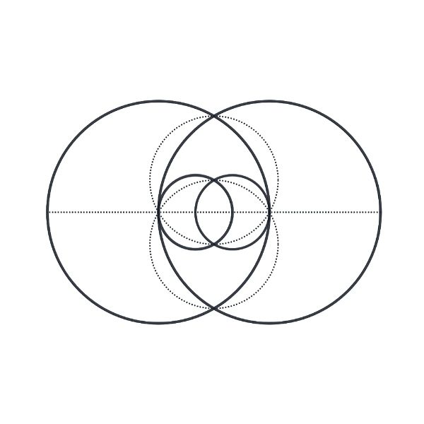
The Vesica Piscis, derived from overlaying two circles with equal diameters, has captivated countless cultures throughout history. This enigmatic symbol, with its intersections and geometric proportions, carries deep sacred meaning and has left an indelible mark on various belief systems and scientific theories. Join us as we delve into the rich tapestry of Vesica Piscis, exploring its origins, symbolism, and its profound implications in both the spiritual and scientific realms.

Overview

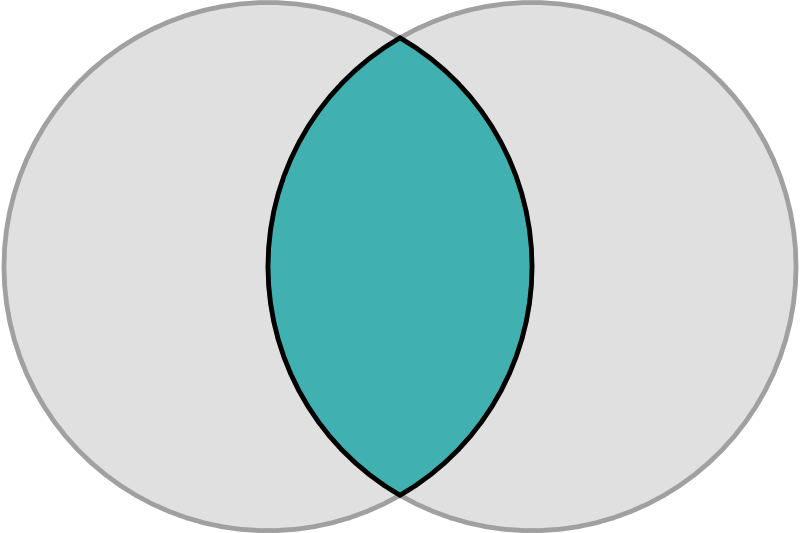
The Vesica Piscis, meaning “fish bladder,” is derived from two circles overlapping in a way that their circumferences touch each other’s centres. The intersectional area is called “mandorla” and resembles an almond. The symbol has origins in Pythagorean history, Christian iconography, and various ancient civilizations. It is associated with the infinite and is used in Venn diagrams. II has implications in Dimensionless Science, and the relationship of the speed of light to the speed of sound.  It can be seen to represent the emission of electromagnetic waves to paired electrons, and is found in the shape of deep space nebulae. Overall, the Vesica Piscis shapes the foundations of the universe.

InInfinity SacredGeometryWorkshop VesicaPiscis TheEyeofGod

A Sacred Symbol with Diverse Origins

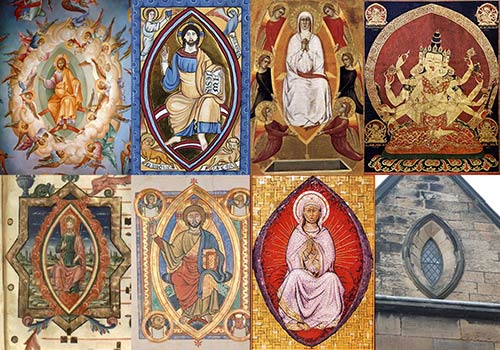
The exact roots of the Vesica Piscis symbol remain elusive. From Pythagorean Greece to Ancient Egypt, Mesopotamia, India, China, and Africa, this symbol has transcended time, manifesting in different cultures across continents. In Ancient Greece, it was revered as the Ichthys, symbolizing the creation of the Syrian Goddess Atargatis. Celtic and Norse cultures associated it with the divine feminine and the vulva of goddesses. In Christian art, notably linked to Mary Magdalene, the Vesica Piscis has been depicted as a representation of the Cosmic Mother.

Universal Symbolism of Infinity

The circle, universally recognized as a symbol of the infinite and perfection, finds its expression in Vesica Piscis. With no vertex, no beginning, and no end, the circle embodies limitless potential and divine essence. The Vesica Piscis, formed by two intersecting circles, takes this symbolism further with its sacred geometry, portraying unity, creation, and the convergence of celestial forces.

Exploring its Geometric Proportions

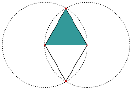
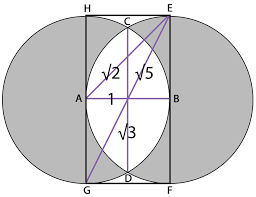
The geometric aspects of the Vesica Piscis hold both beauty and profound mathematical implications. Two contiguous equilateral triangles can be inscribed within the Vesica Piscis, revealing the relationship between vertical and horizontal proportions as 1:√3. We also find √2 and √5, are encoded into its structure, which are the genesis for the creation of the Silver and Golden ratios.

If the side of the triangle is 1,  the distance between tips is √3.
Within its structure, We also find the ratio √2 and √5

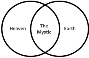
This fascinating ratio finds its way into numerous architectural marvels and even permeates Venn diagrams, challenging the traditional notion that 1+1 equals only 2.

1+1=3
If the side of the triangle is 1, then the distance between each tip is √3.

Scientific Significance

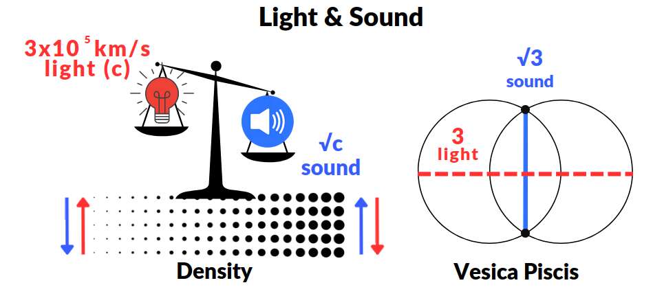
Beyond its spiritual connotations, the Vesica Piscis also plays a significant role in scientific realms. The Geometric Universe Theory, which employs dimensionless science, correlates the dimension of the Vesica Piscis through the horizontal with the speed of light set to 3. This dimension is intricately linked to the maximum speed of sound found in an infinitely dense medium, as observed in baryonic acoustic oscillations (BAOs) within the cosmic microwave background.

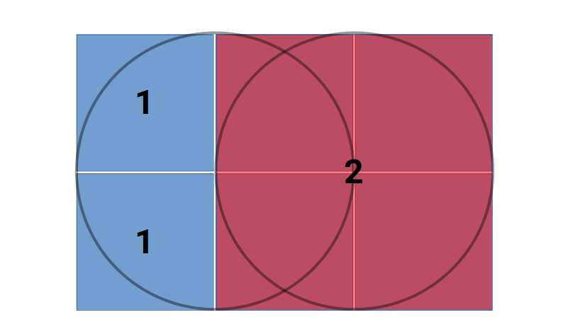
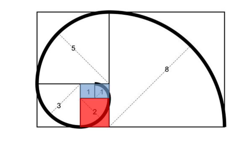
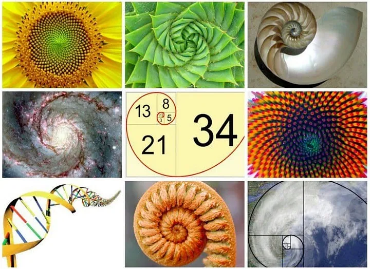
Vesica Piscis and the Fibonacci spiral

The Vesica Piscis fits perfectly within a 2 by 3 rectangle. This also initiates the Fibonacci spiral, which is observed in a wides range of natural phenomena. From flower formations to fruit, to the proportions of a wide range of lifeforms, and even galactic spiral, the Fibonacci appear to structure the domain of matter.

Fibonacci numbers = 1, 1, 2, 3, 5, 8, 13, 21, 34, 55, 89, 144…
Fibonacci numbers in nature

From the Microcosmic to the Macrocosmic

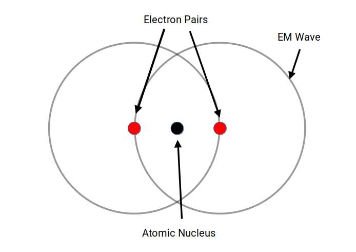
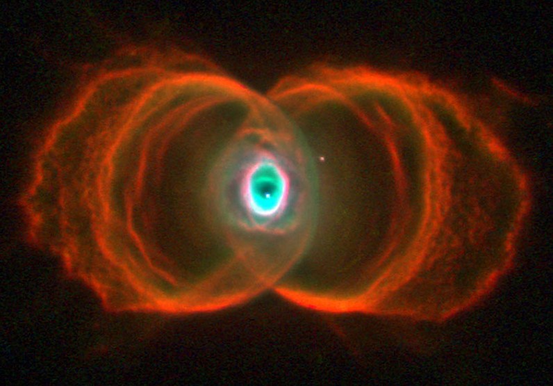
The Vesica Piscis’ influence spans from the microcosmic realm to deep space. Electrons, forming pairs with up and down spins, release electromagnetic waves when transitioning to lower energy states, which can be represented by the Vesica Piscis. This symmetrical pattern also manifests in the awe-inspiring appearance of deep space nebulae. Thus, from the foundational building blocks of atoms to the expanse of the universe, the Vesica Piscis continually shapes and influences our cosmic existence.

THE

Conclusion

Divider Menu

The Vesica Piscis stands as a powerful and timeless symbol that has transcended cultural and religious boundaries throughout history. From its mysterious origin to its representation in art, science, and the cosmic realm, this symbol continues to captivate our collective imagination. As we delve into the interconnectedness of the universe, the enduring presence of the Vesica Piscis serves as a reminder of the underlying unity and profound mysteries awaiting our exploration.

Carry on Learning

Discover more about SACRED GEOMETRY
DIVIDER BLACK
platonic solids

Platonic Solids

Create the 5 Platonic Solids More info Only 5 regular solids in 3D Just as 2D space is limited to only 2 types of regular 2D tessellation that can fill a plane with just two colours, there are only five regular solids. These Platonic Solids have the characteristic of being

Read More »

Quadrivium

The Quadrivium, a fundamental component of the Seven Liberal Arts, encompasses four key disciplines: Mathematics and Science, expressed through Geometry, Music, Cosmology, and Pure Number. Rooted in the teachings of eminent philosopher Plato, this ancient concept emphasizes the importance of studying numbers as a means to unravel the hidden principles

Read More »

Symbol

Sacred Geometry Symbols These are all the spiritual and religious symbols from Islam, Christianity, Judaism to Buddhism, Hinduism, Jainism and Taoism. Most symbols are being shared between the different religions, yet most are known to be related to a specific religion.

Read More »