Introduction
Atomic Geometry is a geometric model of the atom that maps the four orbital types — S, P, D, and F — onto Platonic and Archimedean Solids nested perfectly inside one another. It produces a 3D model of every stable element on the periodic table that is significantly more accurate than the Bohr model — over 500% more accurate for helium, for example — and requires no equations, only geometry.
Where all previous models of the atom have been built from energetic data, Atomic Geometry asks what geometry underlies those patterns. The results reveal that the electron cloud is not a probabilistic blur but a highly ordered geometric structure.
Key takeaways
- The four orbital types (S, P, D, F) map directly onto Platonic and Archimedean Solids — a geometric sequence that predicts atomic radii more accurately than the Bohr model and explains electron configuration without probability theory.
- The electron cloud is not a probabilistic particle but a 4D toroidal field: the up/down spin of electron pairs, the octahedral symmetry of P-orbitals, and the cubic symmetry of D-orbitals all emerge naturally from 4D geometric principles.
- Atomic Geometry can be physically constructed — using nothing more than a compass, ruler, card, scissors, and glue — making advanced quantum concepts accessible to learners of any age.
Watch: Atomic Geometry Overview
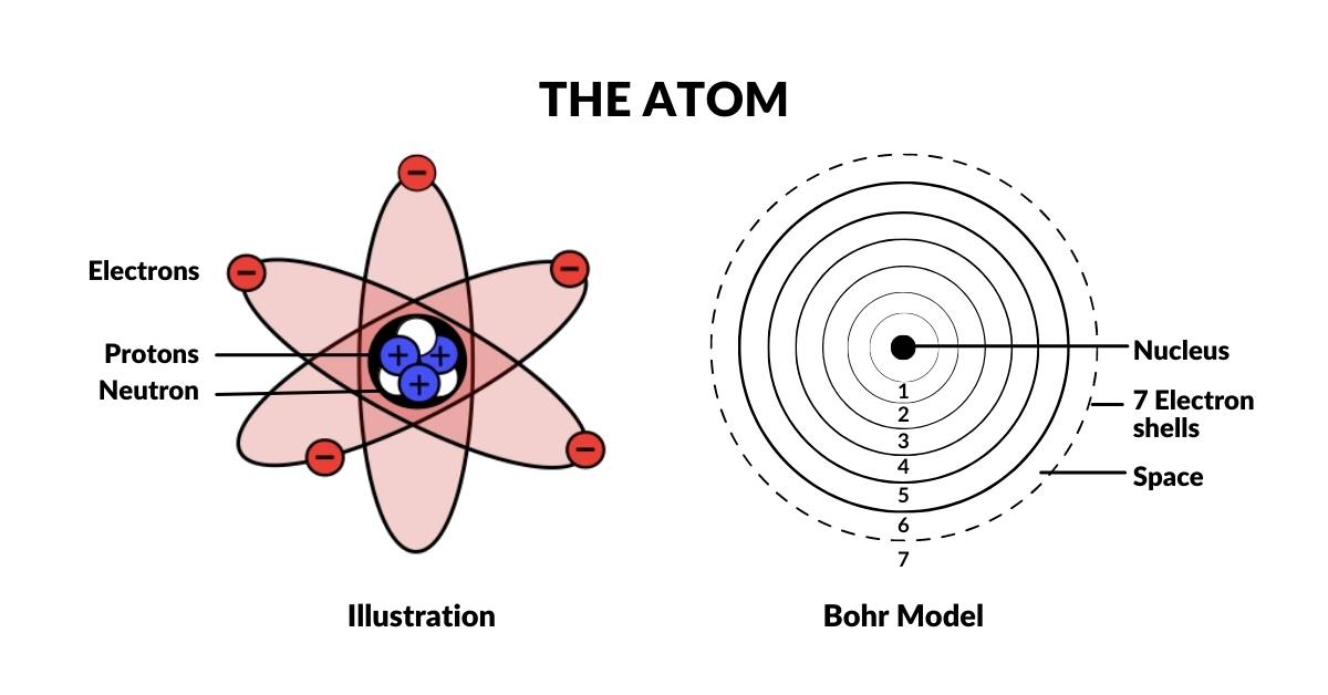
The Atom
Almost everyone knows that matter is made of atoms. Each atom has a nucleus of protons and neutrons accounting for over 99.99% of the atomic mass, surrounded by an electron cloud that falls into distinct shells at specific distances from the nucleus. There are only 6 main orbital shells that make up all stable atoms — the 7th being naturally radioactive.
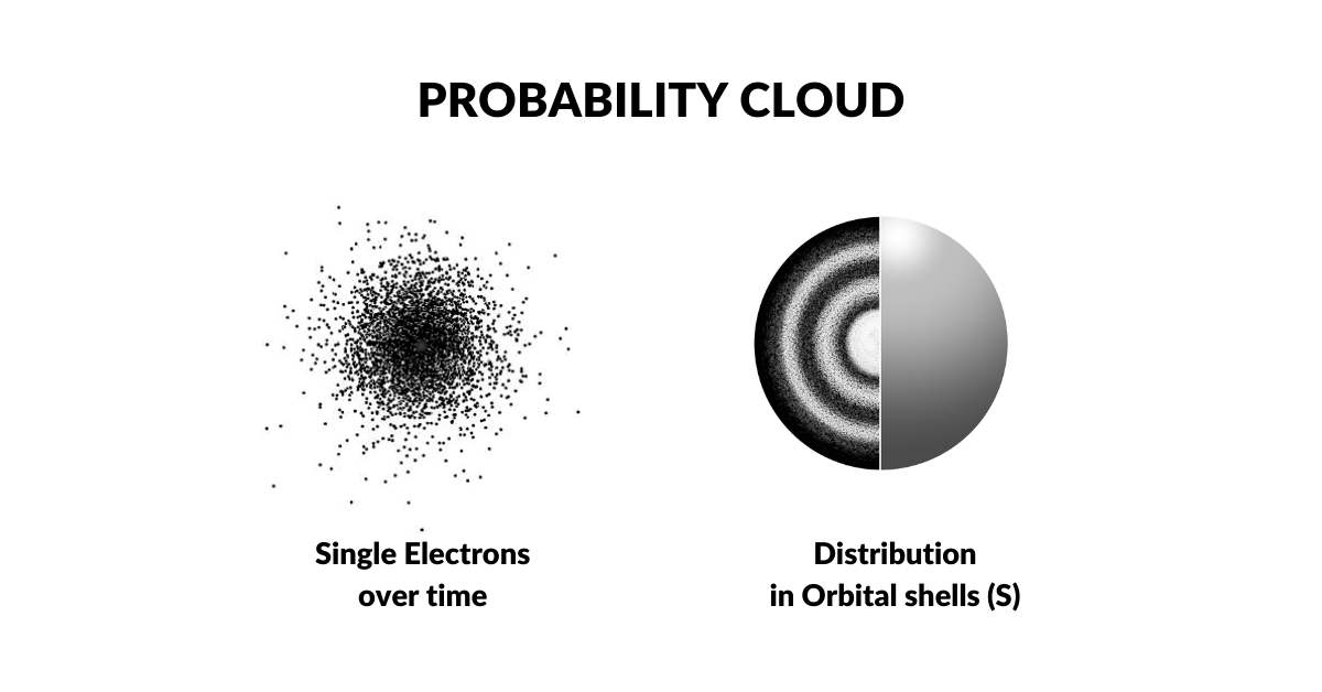
The Electron Cloud
The Bohr model was overturned in the 1920s when Louis de Broglie discovered that electrons exhibit wave-like characteristics. This led Werner Heisenberg to propose that electrons exist as a wave of probability — a notion supported by the fact that the electron's exact location defies measurement. The act of measurement itself was said to collapse the wave into a particle. This established the electron cloud as a function of probability: the Copenhagen Interpretation, which remains the dominant model today.
The idea that the electron might not be a particle has rarely been explored by the mainstream. Yet our wave solutions to the Ultraviolet Catastrophe and the Photoelectric Effect demonstrate that the photon particle proposed by Einstein is not required — both phenomena can be resolved with a pure wave model. Applying the same logic to the electron cloud, it can be understood not as a particle but as a 4D field of energy — dissolving the wave-particle paradox and removing the need for probability theory.
For more on the wave-based alternative, see Is there an alternative to wave-particle duality?
Electron Orbitals
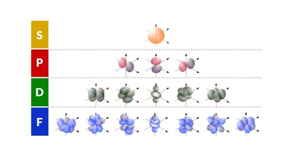
The S, P, D, and F orbitals define precise spaces around the nucleus. Current quantum wave mechanics has noted their relationship to spherical harmonics, but despite consistent experimental evidence no clear geometric conclusion has ever been drawn — until now.
Electron Configuration
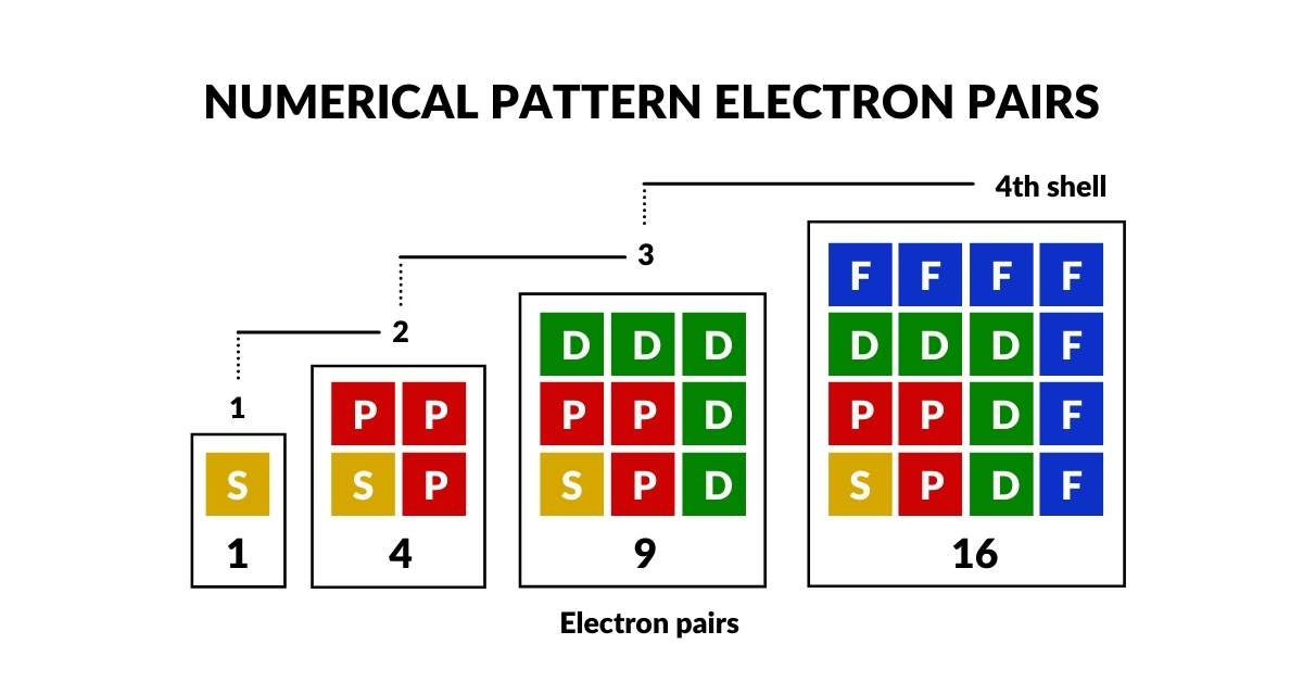
The sub-orbitals appear in a specific order and number — the Electron Configuration. S-orbitals appear once per shell; P-orbitals in sets of 3; D-orbitals in sets of 5; F-orbitals in sets of 7. The pattern 1, 3, 5, 7 is an odd-number series that falls naturally into a triangular formation — the first geometric insight into atomic structure.
When the orbital pairs per shell are totalled, the pattern 1, 4, 9, 16 emerges — a square-number series (1², 2², 3², 4²). The maximum number of electron pairs in a single shell is 16.
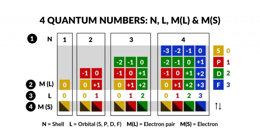
The four quantum numbers — a geometric reading
Each electron's state is defined by four quantum numbers. Atomic Geometry gives each a geometric meaning:
- N = 1–7 (shell / energy level) → geometric nesting depth
- L = 0, 1, 2, 3 (S, P, D, F) → Platonic or Archimedean Solid type
- Mₗ = −L…L (orbital orientation) → face or axis of the containing solid
- Mₛ = ±½ (spin) → north/south pole of the 4D torus field
2D Orbital Geometry
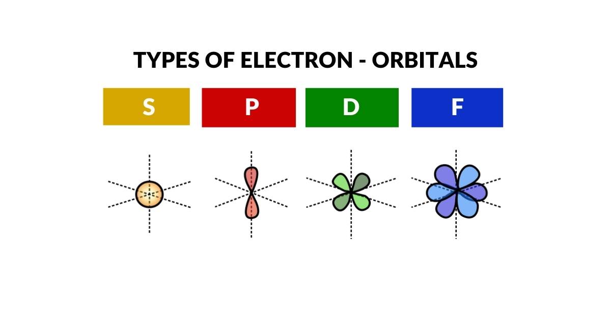
When we examine the shapes of each sub-orbital, the geometry deepens. S-orbitals are spherical. P-orbitals divide the sphere into two lobes — one up, one down. D-orbitals divide again to form a cross. When it comes to F-orbitals, the pattern shifts to a hexagonal arrangement. This progression — sphere, line, cross, hexagon — corresponds exactly to the four geometric primitives constructible from regular 2D tessellation. For more on this, see 2D Orbital Geometry of the Electron Cloud.
3D Orbital Geometry — The Platonic and Archimedean Solids
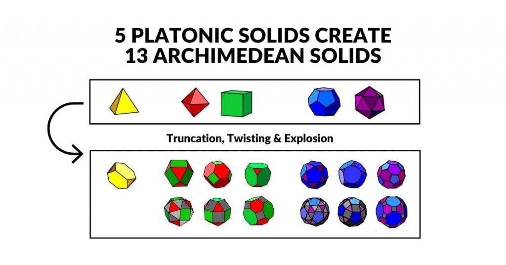
Each sub-orbital comprises a specific number of lobes to form a complete 3D set. In 3D, Atomic Geometry maps these sets onto the five Platonic Solids and thirteen Archimedean Solids — the only regular and semi-regular polyhedra in three dimensions.
Comparison with Other Atomic Models
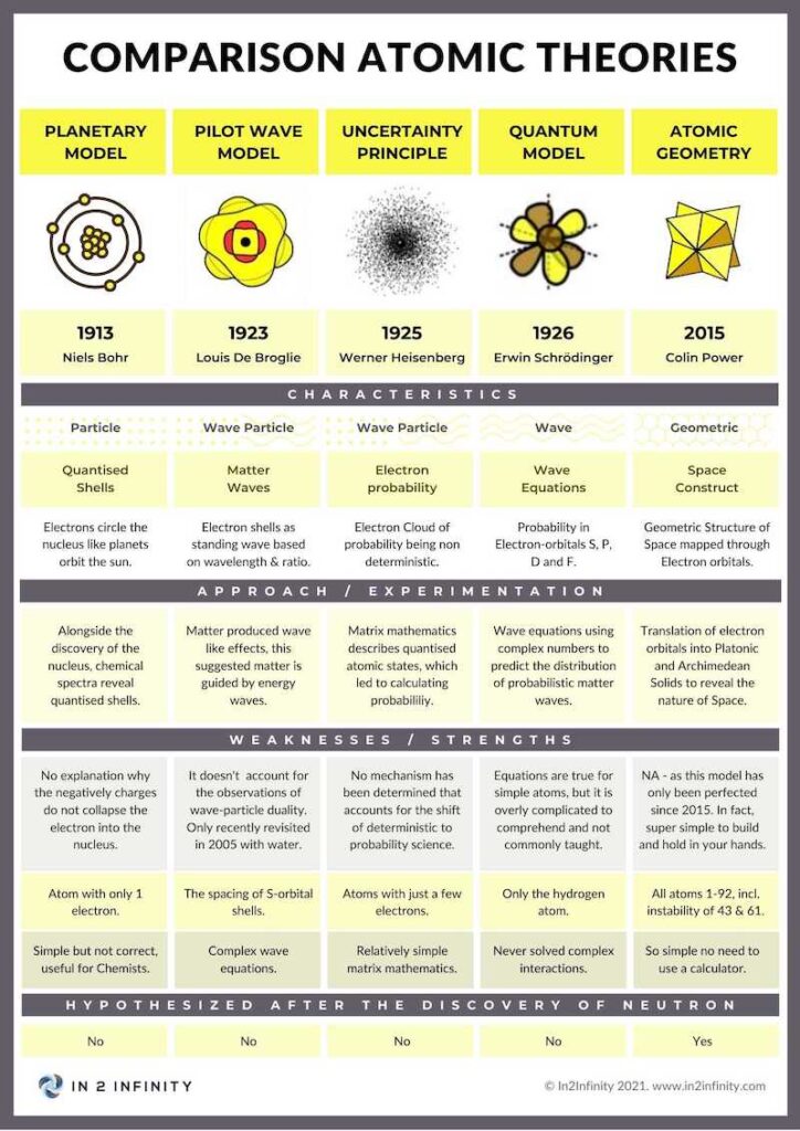
Atomic Geometry shares common ground with existing models while resolving several longstanding problems. Unlike the Copenhagen Interpretation, it treats the orbital as a definite geometric form rather than a probability cloud. Unlike Pilot Wave theory, it does not require a non-local guiding field. Unlike the MCAS model, it grounds orbital shapes directly in the Platonic and Archimedean Solids rather than algebraic curve-fitting.
S-Orbitals
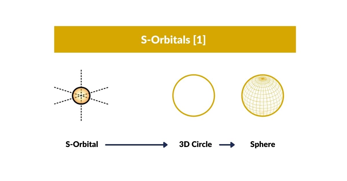
The spherical S-orbitals are the first to appear in every atom. Each consists of two electrons oriented in opposite directions — up and down. S-orbitals play a key role in simple atomic bonds, appearing first on the outermost valence shell.
S-Orbitals and the Torus
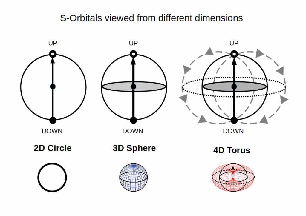
S-orbitals can be perceived as a circle (2D), sphere (3D), or torus (4D). In 4D, the two electrons follow the flow of the toroidal field — a dynamic structure in continuous motion, exhibiting a unidirectional energy flow from the down-oriented electron, through the nucleus, to the up-oriented electron. This is why electron pairs always appear as opposites: they are the two poles of a 4D torus field.
For the detailed treatment, see S-Orbital Geometry.
P-Orbitals
After the first four elements, the first P-orbitals appear. Starting with boron (5), this set includes the building blocks of biological life — carbon (6), nitrogen (7), and oxygen (8). All noble gases (except helium) occur when a full set of six P-orbital electrons completes the shell.
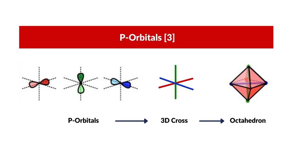
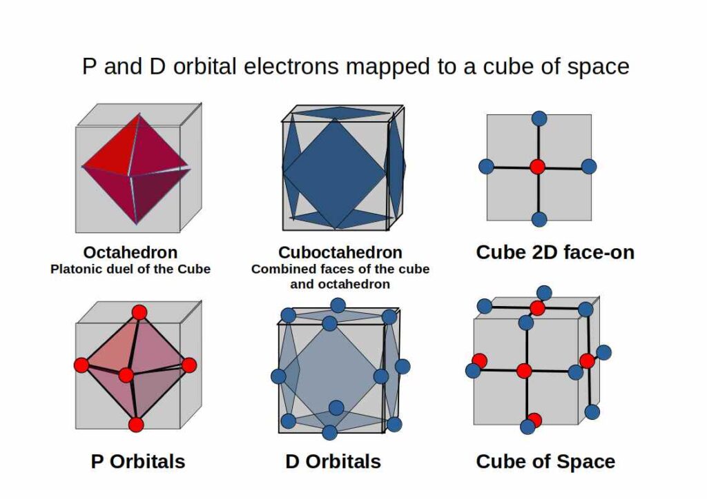
P-Orbitals and the Octahedron
P-orbitals always appear in sets of three, each orientated at 90° to the others, forming a 3D cross spanning x, y, and z. Superimpose an Octahedron over the centres of the three P-orbitals and it fits perfectly — making the Octahedron the defining solid of the noble gas configuration and the foundation for the octet rule.
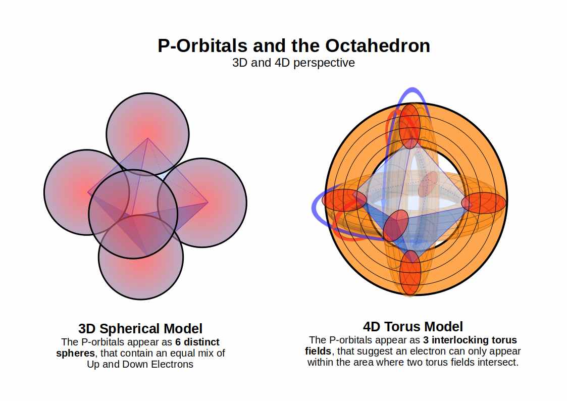
4D P-Orbitals
In 4D, each P-orbital lobe connects to the other through a torus ring, so the complete set of three P-orbitals resembles three interlocking torus fields mapped onto an Octahedron rather than the simple dumbbell shape of the 3D model.
Watch: P-Orbitals as an Octahedron
The octahedral geometry of the P-orbitals also provides a framework for understanding the noble gases — the non-reactive elements that complete each orbital shell. Through the jitterbug transformation and dodecahedral nesting, the geometric model predicts noble gas radii and offers an explanation for their chemical inertness based on the inability of pentagonal geometry to fill space. For the detailed treatment, see P-Orbital Geometry.
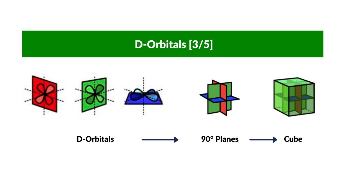
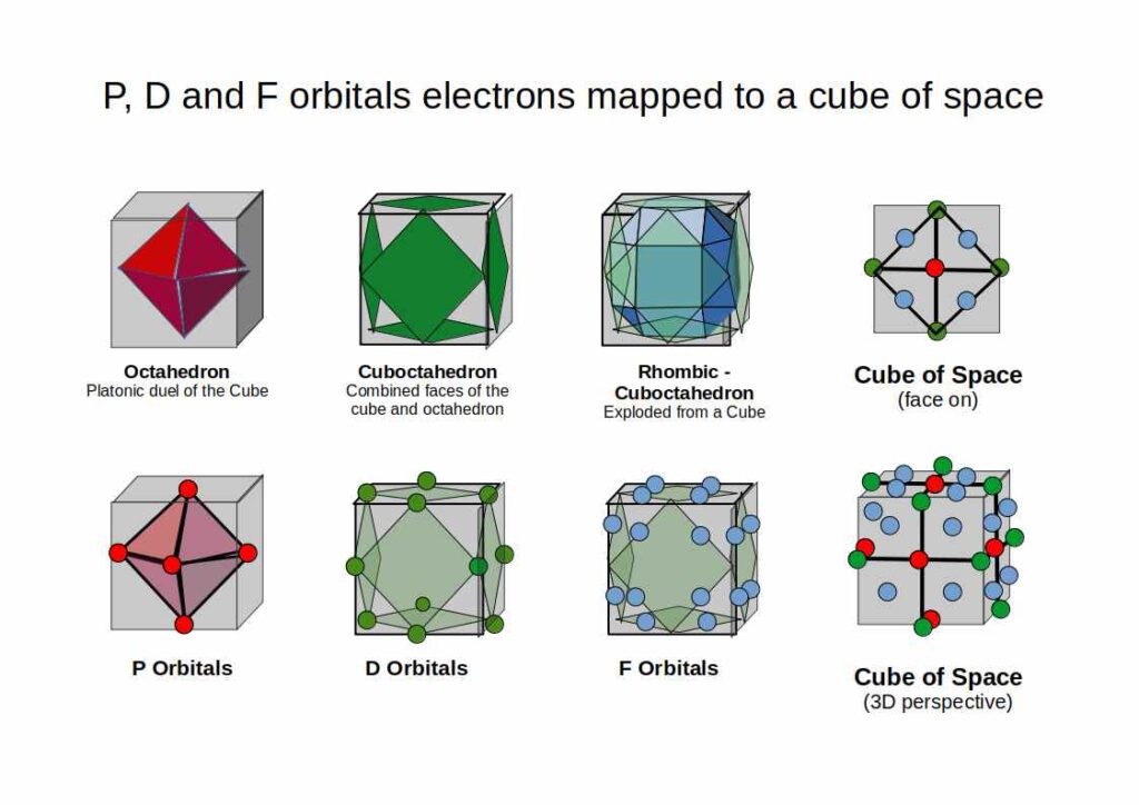
D-Orbitals
Building on the P-orbital Octahedron, D-orbitals extend the geometry into cubic space. Three of the five D-orbitals share the same x, y, z axis as the P-orbitals and divide a cube of space into eight equal parts. The remaining two map onto the Rhombic-Cuboctahedron — the only Archimedean Solid whose midsection can rotate freely, matching the toroidal dynamic of the final D-orbital pair.
D-Orbitals — dx²-y² and dz²
The remaining two D-orbitals complete the set of five. The dx²-y² orbital places four lobes directly along the x and y axes — rotated 45° relative to the dxy orbital. The dz² orbital is unique: two lobes along the z-axis plus an equatorial torus ring, mapping onto the Rhombic-Cuboctahedron — the only Archimedean Solid with a freely rotating midsection, matching the toroidal dynamic of this orbital.
There are three stable sets of D-orbital elements. Each set maps to a progressively higher-dimensional polytope, explaining Aufbau anomalies, ferromagnetism, and electrical conductivity through geometry rather than energy rules alone. The reciprocal space of the atomic lattice — known as Brillouin Zones — reveals that magnetic elements (iron, cobalt, nickel) express a Rhombic-Dodecahedron, while conductive elements (copper, silver, gold) express a Truncated Octahedron. For more on this geometric connection, see Brillouin Zones and the Geometry of Ferromagnetic and Conductive Waves.
For the full treatment of D-orbital geometry see D-Orbital Geometry Part 1, Part 2, and Part 3.
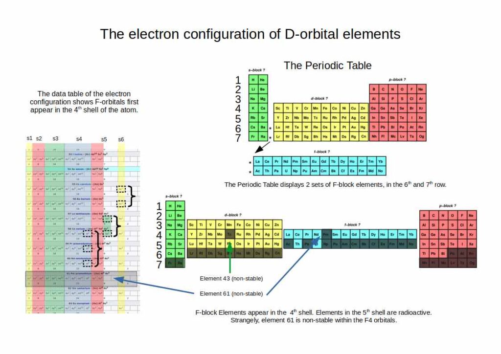
F-Orbitals
F-orbitals appear spatially in the 4th shell, though the periodic table places them in the 5th and 6th rows because elements are ordered by energy level. Only one set is stable (elements 57–71); the second set is radioactive.
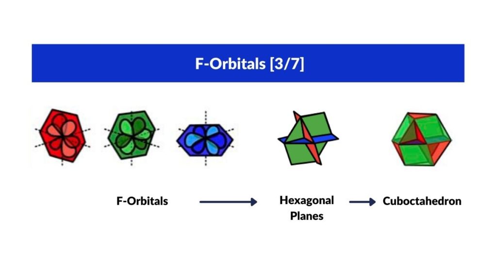
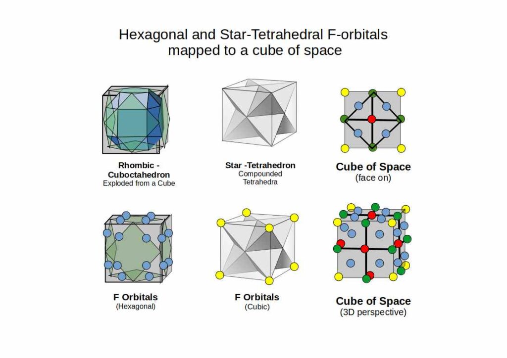
F-Orbitals and the Cuboctahedron
The most common F-orbital configuration is hexagonal. Four hexagonal rings orientated along x, y, and z fit the Cuboctahedron perfectly — which has both square and triangular faces, with an internal geometry of four hexagons. The full orbital sequence is: Octahedron (P) → Cube (D) → Cuboctahedron (F).
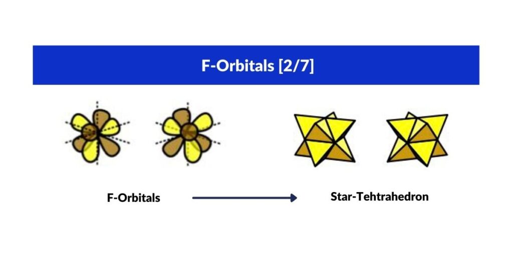
F-Orbitals and the Star-Tetrahedron
Within the F-orbitals there is one unique cubic-shaped pair: each electron contained within a Tetrahedron, the two interlocking at 180° to define the corners of a Cube. This is the Star-Tetrahedron — an Octahedron with eight tetrahedra on each face. Just as P-orbitals begin atomic structure with an Octahedron, F-orbitals terminate it with the Star-Tetrahedron.
F-Orbitals and the √2 Fractal
The star-tetrahedral orbitals locate at each corner of the cube. Viewed from the centre face, the electron distribution is limited to the corner points of nested squares, each successive square differing in size by a factor of 1:√2. This √2 fractal is also found in the geometry of electromagnetic waves — and explains why one set of D-orbitals is offset by 45°.
F-Orbital Torus and the Icosahedron
The final F-orbital is a double torus — a 5D hypersphere assigned to the Icosahedron. Like the Rhombic-Cuboctahedron among the Archimedean Solids, the Icosahedron has a rotational property: deconstructed into three sections it reveals a pentagonal middle prism containing the Golden Ratio (1:1.618, related to √5).

The Jitterbug Transformation
The geometric progression from S-orbitals through to F-orbitals is not a coincidence — it is driven by a single geometric mechanism. The jitterbug transformation, first described by Buckminster Fuller, shows how the cuboctahedron can collapse through the icosahedron and octahedron to the tetrahedron. This same transformation connects each orbital type to the next, explaining why the electron cloud builds in the specific sequence it does.
Conclusion
Atomic Geometry provides a clear, geometrically rigorous description of the atom. Where standard models invoke probability and wave-particle duality, it offers a deterministic geometric alternative — one that is more accurate, simpler to grasp, and physically constructible.
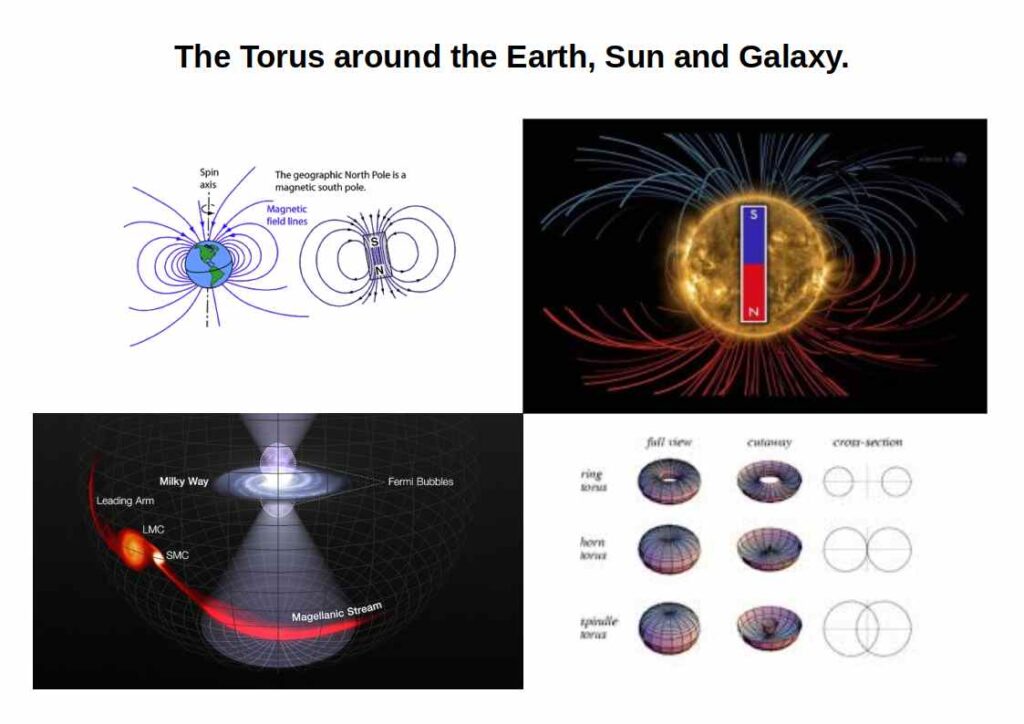
The orbital sequence S → P → D → F is not arbitrary. It is a geometric progression: torus → Octahedron → Cube → Cuboctahedron — each step adding a dimension, each form nesting inside the last. The geometry is not merely three-dimensional: orbitals exist in the fourth dimension and possibly the fifth, based on the Euclidean axioms of 1D through 5D rather than on string theory. The same toroidal and hypercubic structures that define the electron cloud appear at planetary, stellar, and galactic scales — suggesting a single geometric principle operating at every level of reality.
Atomic Geometry is compatible with the Copenhagen Interpretation and the de Broglie Pilot Wave model, but extends both by offering a mechanism — geometry — where they offer only description. It connects naturally to Geo-Quantum Mechanics, Dimensionless Science, and the 4D Aether framework.
For the detailed article series: History of the Atom · The 4D Electron Cloud · S-Orbital Geometry · P-Orbital Geometry · D-Orbital Geometry (parts 1, 2, 3) · 2D Orbital Geometry · The Atom and the Seed of Life · Brillouin Zones
FAQ
Why hasn't science recognised the geometric nature of the atom?
We have approached the scientific community with these ideas. The geometric model's simplicity may work against it — quantum mechanics is generally associated with complicated mathematics, and a model that can be grasped without equations can seem too easy to take seriously. We continue to develop the quantitative side of the theory alongside the geometric presentation.
Is this model applicable to all elements on the periodic table?
Data about the S, P, D, and F orbital shells has been gathered by energising a hydrogen atom, which science uses as the simplest case. As hydrogen has no neutron, atomic radii change across the periodic table. Our more advanced model, Geo-Quantum Mechanics, produces predictions of atomic radii that more closely match experimental values than the Bohr model across all stable elements.
How accurate is Atomic Geometry compared to the Bohr model?
For elements such as helium, the Atomic Geometry model predicts atomic radii over 500% more accurately than the Bohr model. The geometric approach outperforms energy-based models because it works from the spatial structure of the electron cloud rather than fitting equations to observed energy levels.
Can children understand Atomic Geometry?
Yes — children as young as seven have recognised concepts such as electron configuration, orbital shells, and electron pairing when introduced through the geometric model. Because it can be physically constructed with a compass, ruler, card, scissors, and glue, it becomes a tactile experience rather than an abstract mathematical one.
What does Atomic Geometry say about wave-particle duality?
Atomic Geometry treats the electron not as a particle with a probabilistic location but as a 4D field of energy whose quantised states are defined by the geometry of fourth-dimensional polytopes. This removes the need for probability theory to describe the electron cloud and resolves wave-particle duality at its source — the same resolution proposed in our 4D wave model of matter.