P-orbital Geometry

Introduction

P-orbitals are the second type of orbital to appear in the atomic structure, after the spherical S-orbitals. Where the S-orbital forms a single sphere around the nucleus, each P-orbital consists of two lobes positioned on either side of the nucleus, like a dumbbell. They always appear in sets of three, oriented along the x, y, and z axes — six lobes in total, forming an octahedral arrangement around the atom's centre.

P-orbitals first appear in the second shell of the electron cloud and are responsible for the chemical behaviour of many familiar elements, from the carbon, nitrogen, and oxygen that make up biological life to the silicon and germanium at the heart of modern electronics. Understanding their geometry is key to understanding why these elements behave the way they do.

In this article, part of the Atomic Geometry series, we explore how the geometric ratios of nested polyhedra — particularly the octahedron and cuboctahedron — predict the radii of P-orbital elements with remarkable accuracy. For background on how the electron cloud is structured, see The 4D Electron Cloud, and for the historical context, History of the Atom.

What is a P-orbital?

The electron cloud surrounds the atomic nucleus and is composed of different shells, each found at a specific distance from the centre. In the simplest picture — the Bohr model — these shells are drawn as concentric rings, each holding a certain number of electrons. Once a shell is filled, subsequent electrons begin to fill the next. This model is still widely used in introductory chemistry, but a more accurate description comes from the S, P, D, and F orbital model, derived from the Schrödinger equations (see also wave-particle duality). This reveals that each shell is composed of up to four different orbital types, each with its own distinct geometry.

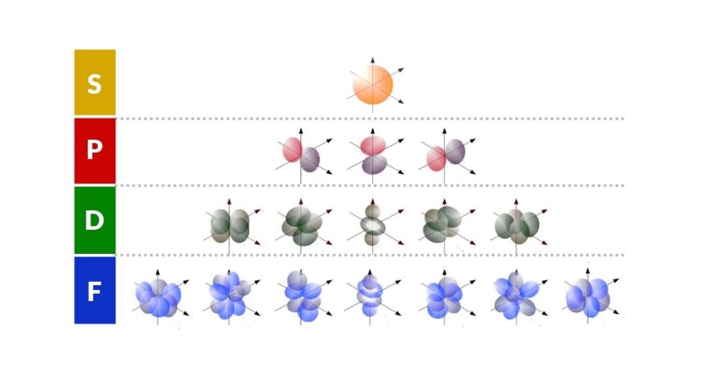
The S-orbital is a sphere. The P-orbital, by contrast, has a distinctive two-lobed shape — and because three P-orbitals are oriented at right angles to each other, their six lobes point to the six corners of an octahedron. This octahedral arrangement is the geometric foundation upon which the rest of this article builds.

Cuboctahedron and the P-orbitals

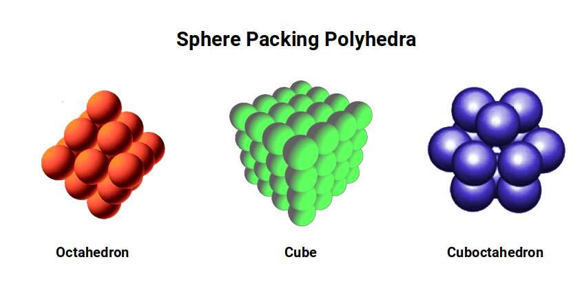
The faces of a cube and octahedron can be combined into a single polyhedron called the cuboctahedron. This Archimedean solid is unique: its adjacent corners are the same distance from each other as they are from its centre, which is why it is sometimes called the vector equilibrium. It is the ideal shape for nesting spheres in 3D space — a configuration known as hexagonal close packing. Together with the cube and octahedron, these three shapes produce almost all known crystalline atomic structures.

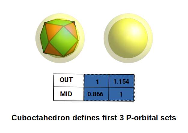
The cuboctahedron has an out-sphere (touching its corners) and a mid-sphere (touching its edges), plus two types of in-sphere due to its square and triangular faces. With an out-sphere radius of 1, the mid-sphere has a radius of 0.866. This ratio defines the difference between the beginning of the first P-orbital set and the end of the second. If the mid-sphere is set to 1, the out-sphere measures 1.154 — defining the difference between the end of the second and third P-orbital sets.

The first and second P-orbital radii reduce to 0.5 Å and 1 Å respectively, a 1:2 ratio. This doubling pattern is expected from sets of nested octahedra. After the second set, the first D-orbitals appear (elements 21–30), before the third P-orbital set begins (elements 31–36). This seems to break the doubling pattern: instead of reaching a radius of 2, the third set settles at an average of 1.154. The D-orbitals generally fall at a radius of around √2 (1.4 Å), which constrains the third P-orbital set. The first element in this set, gallium (31), has a radius of 1.3 Å, followed by germanium (32) at 1.25 Å, after which the next three elements all share a radius of exactly 1.154 Å. The cuboctahedron's out-sphere to mid-sphere ratio perfectly defines this spacing.

When we extend the nesting pattern and include both types of in-sphere, a mid-sphere of 1.154 produces an out-sphere of 1.333 — extremely close to the radius of gallium (31), well within the margin of experimental error. The radius of germanium (32), 1.257 Å, also appears in the mid and in-spheres of the cuboctahedrons above.

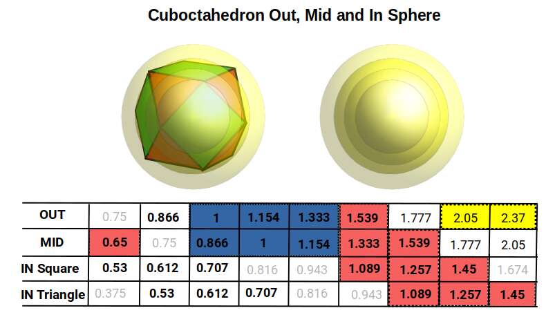
The highest numbers in this dataset roughly define the radii of the S-orbital pair that forms between the third and fourth P-orbital sets: rubidium (37) at 2.3 Å and strontium (38) at 2 Å (highlighted in yellow). All D-orbital elements fall between 1.55 Å and 1.3 Å (highlighted in green), defined by the out-sphere and mid-sphere of the third iteration above 1. (The geometric properties of these D-orbital elements also explain their ferromagnetic and conductive behaviours — see Brillouin Zones.) The F-orbital sets, with two main radii of 1.85 Å and 1.75 Å, are also approximately defined by a value of 1.777 (highlighted in blue).

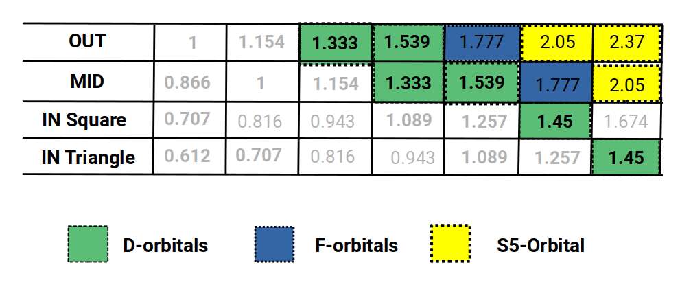
Reading the chart diagonally reveals the radii for all P-orbital sets. The fourth set starts with indium (49) at 1.55 Å, falling to 1.45 Å for the two subsequent elements. This increase in radius, unexplained by the octahedral model alone, is accounted for in the cuboctahedral dataset.

The third set similarly falls from 1.3 Å to 1.25 Å before settling at 1.154 Å — again, values found in the cuboctahedral model. The same applies to the second P-orbital set: aluminium (13) at 1.25 Å, silicon (14) at 1.1 Å, then settling at 1 Å. The cuboctahedral dataset produces values of 1.257, 1.089, and 1 — a very close match. Finally, the first P-orbitals show radii of 0.866, 0.707, 0.65, 0.612, and 0.53, all well within the margin of experimental error.

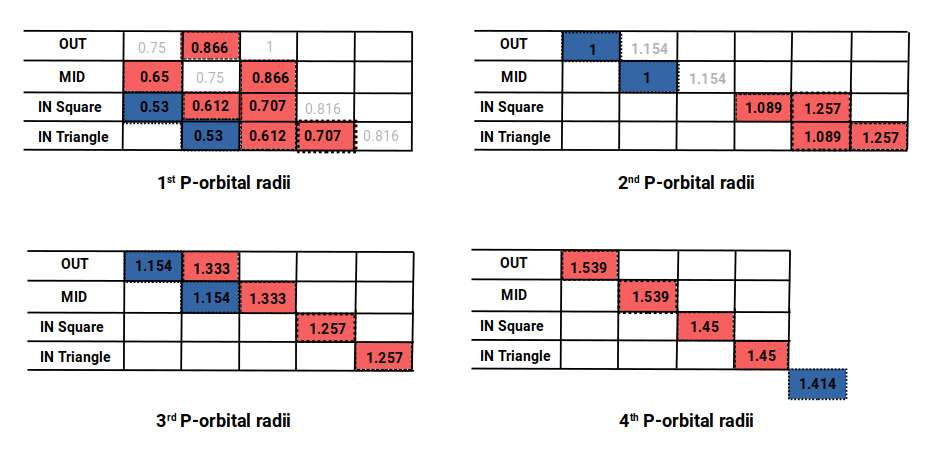
The last P-orbitals finish with a radius of √2, which does not appear in the cuboctahedral set but is found in the cubic and octahedral models. When this dataset is compared to the experimentally determined radii and the Bohr model, the geometric model proves to be an almost exact match for the experimental data.

In summary, the cuboctahedral space explains how the P-orbitals transition from the S and D-orbital types as each lobe fills with electrons, resolving anomalies found in the octahedral and cubic models alone. The cuboctahedral model expands at a rate of 2÷√3 — a value also found as the ratio between a cube's side length and the distance to its vertex. Combined with the other ratios of the cube and octahedron (1, √1.5, √2, and √3), these geometric relationships define the radii of every stable element on the periodic table — a closer match to experimental data than the Bohr model provides.

It is worth noting that this is not a case of fitting arbitrary parameters to data. The polyhedra used — octahedron, cube, cuboctahedron — are not chosen freely but are geometrically constrained: each one nests inside the next through fixed mathematical relationships. The ratios emerge from the geometry itself, not from adjusting values to match observations. The model uses only four fundamental ratios (1, √1.5, √2, and √3), all derived from the same family of polyhedra, to predict the radii of over 80 elements. This is what distinguishes it from curve fitting: the geometric structure predicts the data, rather than being shaped by it.

Geonuclear physics of the 1st P-orbitals

The geometric model so far has provided a compelling account of the observed radii across the periodic table. Through octahedral, cubic, and cuboctahedral nesting, we can reproduce all the P-orbital radii and define the range for the D and F orbital elements. These results are observational — the geometric ratios match the experimental data. But we can go one step further by asking why the ratios match, examining each atom as a whole structure — nucleus included.

Geonuclear physics proposes that the protons and neutrons in each nucleus arrange into specific geometric configurations, and that the shape of each nucleus directly determines the radius of the electron cloud. Where the standard S, P, D, and F model is based solely on the hydrogen atom, the geonuclear model expands on this by taking into account the nucleonic count of each element. What follows is a hypothesis — but one that produces testable predictions.

Some elements are only stable when they have more neutrons than protons. Boron (5), for example, is stable with 5 protons and 6 neutrons — a total of 11 nucleons, specifically avoiding 10. The reason for this proton/neutron relationship has no clearly defined theoretical basis in current physics. Geonuclear physics offers a coherent solution founded on geometric principles.

The 11 nucleons of boron (5) can be arranged so that the 5 protons form a tetrahedron — 4 at each corner, with one at the centre — while the 6 neutrons create the corners of an octahedron located at the tetrahedron's centre. A tetrahedron with a side of √2 fits inside a cube with a side of 1, producing an out-sphere of 0.866 and a mid-sphere of 0.5. These values define the radii of boron (5) and fluorine (9).

Carbon (6) has 12 nucleons, filling the 12 corner points of a cuboctahedron. Nitrogen (7) has 14 nucleons — the number of faces on a cuboctahedron — defined by the corners of the rhombic dodecahedron, which is the cuboctahedron's dual. Together they form the octaplex, a 4D polytope.

The rhombic dodecahedron is formed from a compound of a cube and octahedron and produces the template for the 4D hypercube. Represented as two cubes nested inside each other, it has 16 corner points — matching oxygen (8), whose 8 protons and 8 neutrons can each be assigned to one of the two cubes. Fluorine (9) has 19 nucleons, which is the number of points needed to form an octahedron made of 6 smaller octahedra. The extra neutron sits at the centre of the structure, with the remaining protons and neutrons filling the external frame.

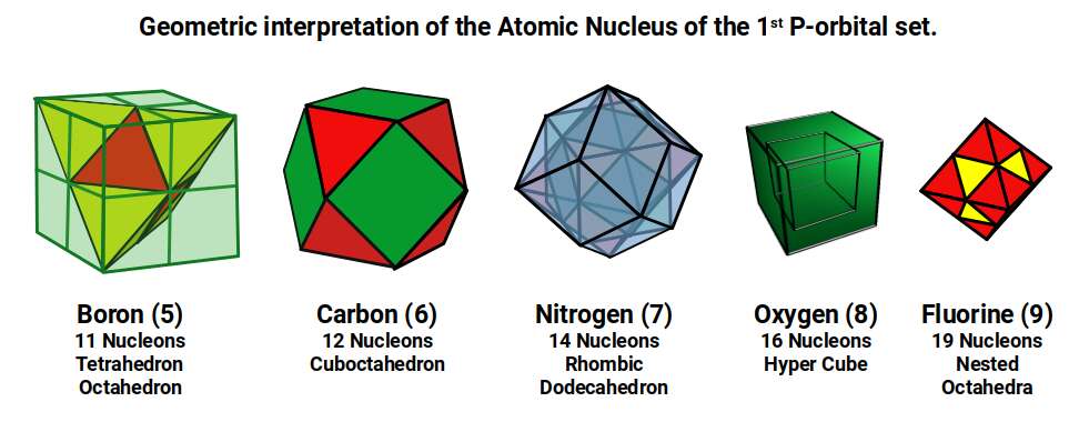
Except for oxygen (8), each of these forms contains an octahedron within its structure. The cube that encloses boron (5) also contains the cuboctahedron of carbon (6). Its dual, the rhombic dodecahedron, contains a second cube and an octahedron. The two cubes form the hypercube of oxygen (8), leaving the single octahedron to form fluorine (9).

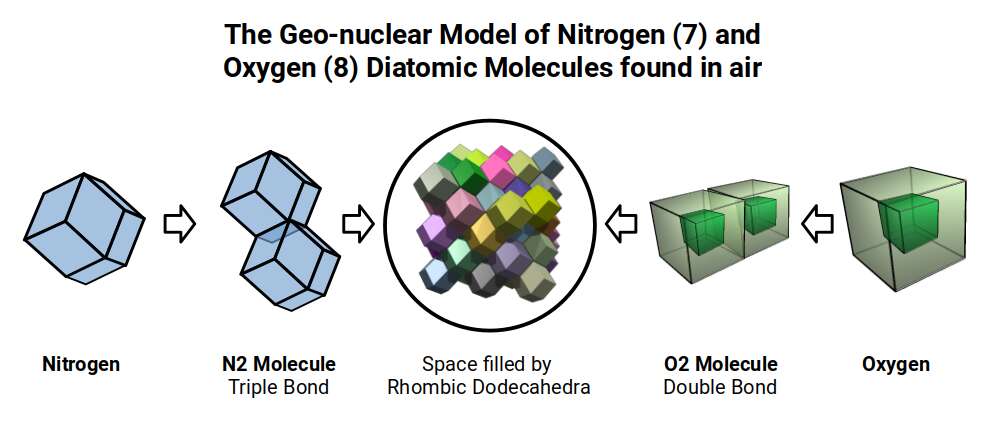
This P-orbital set contains the three elements at the foundations of biological life. Carbon (6) often forms hexagonal rings with other carbon atoms to build cellular structures — and the hexagon is found within the cuboctahedron (a relationship explored further in The Atom and the Seed of Life). Nitrogen (7) and oxygen (8) are unique in the set: they form the diatomic molecules in the air we breathe, achieving this through double and triple bonds that bind two atoms together as a non-reactive molecule. This is unusual, because each molecule has 14 and 16 electrons respectively, whereas non-reactive molecules normally have an electron count of 10 or 18, as found in neon (10) or argon (18). This fact is critical to our ecological and biological systems, yet there is presently no definitive scientific explanation for it.

From a geonuclear perspective, nitrogen and oxygen are the only elements in this set with a hypercubic nuclear structure. The rhombic dodecahedron, like the cube, can fill 3D space — creating the geometric template for the 4D hypercube to manifest. This offers an alternative explanation for the double and triple bonds formed by these two elements.

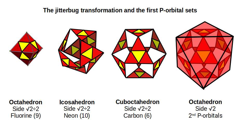
Each of these geonuclear structures contains a relationship to a cube, an octahedron, or both. By setting the side length to a consistent value of √2÷2 (0.707 Å) for each form, the out-sphere almost exactly defines the radii for the entire P-orbital set. (Boron is assigned a side length of √2, double that of the others, so that the octahedron within its structure has a side length of √2÷2.)

The results provide an almost exact match to experimental observations, using only the out-sphere of each shape. This geonuclear model accurately describes the first P-orbital set in terms of radius while simultaneously offering clear explanations for the molecular behaviour of carbon (6), nitrogen (7), and oxygen (8).

The geometry of the noble gases

The transformation of an octahedron into a cuboctahedron can be achieved through a geometric process called the jitterbug. The faces of the octahedron rotate as the form expands, creating gaps that eventually become the square faces of the cuboctahedron. During this process, the spaces first form two equilateral triangles, producing the icosahedron as an intermediate step. Once the cuboctahedron is fully formed, it provides the foundation for another octahedron twice the original size — demonstrating how the octahedral structure doubles, as observed in the first two P-orbital sets.

Up to this point, we have avoided discussing the radii of the noble gases. Because these elements do not form bonds, there is no hard experimental data for their radii. Whether the radius should be smaller or larger than the preceding element remains an open question. The Bohr model, based on the attractive force between electron and proton, predicts a smaller radius. The Van der Waals radius, based on the outermost shell, suggests the radius should increase due to the atom's electrical neutrality.

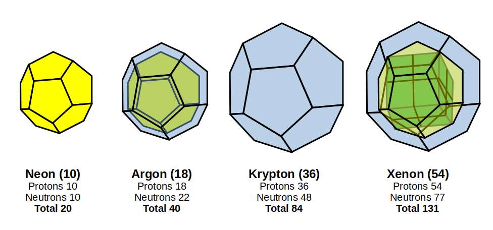
From the perspective of geonuclear physics, we can examine the nucleonic count of the four stable noble gases — neon (10), argon (18), krypton (36), and xenon (54) — and look for geometric correlations.

Note: data is for the most stable isotope of each element.

The number of protons always equals the number of electrons, giving each element its atomic number. However, as elements become heavier, more neutrons are needed to maintain a stable nucleus. This is particularly interesting for argon (18), which has 40 nucleons, whereas potassium (19) — the very next element — has only 39. This anomaly occurs just before the first D-orbitals begin to appear.

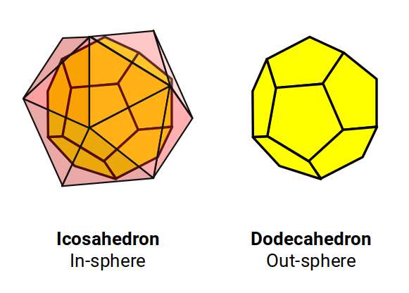
The nucleon count of neon (10) is exactly half that of argon (18), mirroring the 1:2 ratio found between the first two P-orbital sets. Of the five Platonic solids, only the dodecahedron has 20 corner points. Its dual, the icosahedron, can be nested with the dodecahedron's 20 corners touching the centre of each of the icosahedron's faces — exactly the right number to match neon's nucleonic count.

Using the radius of each octahedron from the P-orbital sets, we can produce an icosahedron of the same side length through the jitterbug transformation, then find the in-sphere to define the dodecahedron and predict the sizes of the noble gases.

As a comparison, we can use the Van der Waals radius, which predicts a larger size for the noble gases. Since these radii are generally much larger than experimental values, they need to be scaled. By dividing the Van der Waals radius of a noble gas by that of the preceding element, we obtain a ratio that can be applied to the experimental radius. For example, fluorine (9) and neon (10) have Van der Waals radii of 1.47 Å and 1.54 Å. Dividing 1.54 by 1.47 gives 22/21. Multiplying the experimental radius of fluorine (0.5 Å) by 22/21 produces 0.523 Å for neon. Repeating this for the other noble gases produces results that closely match the dodecahedral model.

The geometric theory offers a prediction based on the nature of the dodecahedron, supported by the nucleonic counts:

• Neon (10): 20 nucleons — one for each corner of a dodecahedron.
• Argon (18): 40 nucleons — exactly double, represented by two nested dodecahedra, analogous to the 4D hypercube.
• Krypton (36): 84 nucleons — the next dodecahedral number after 20 (just as 19 follows 6 in the octahedral number sequence: 6, 19, 44). This can also be composed of two 20-point dodecahedra plus 44 remaining nucleons, which form a third-order octahedron — the correct size to contain the octahedra from the two previous P-orbitals.
• Xenon (54): 131 nucleons — a first and second-order dodecahedron (20 + 84), leaving 27 points that form a cube (3³). This set appears after two sets of D-orbitals, whose cubic nature accounts for the cube within the structure.

The dodecahedral structure of the noble gases offers insight into their non-reactivity. The octahedron, tetrahedron, cube, and rhombic dodecahedron can all fill space, creating larger versions of themselves at each step. The cuboctahedron unifies these shapes and provides the ideal arrangement for sphere packing. The tetrahedron, octahedron, and cube form a set that extends into infinite dimensional space. The icosahedron and dodecahedron, however, appear only in the third dimension, with an analogue limited to the fourth.

These forms contain pentagons, which — unlike squares and triangles — cannot tile the 2D plane perfectly. Instead, two side lengths are required, in proportion to each other through the golden ratio, creating a pattern that expands in scale from a central point rather than repeating uniformly. This geometric property provides an alternative explanation for the inert nature of the noble gases: their dodecahedral structure simply does not fit into the fractal, space-filling geometry that extends into infinite dimensions.

This makes the noble gas radii a direct testable prediction of the geometric model. To date, no experimental technique has precisely determined the atomic radius of the heavier noble gases such as krypton (36) or xenon (54), because they do not form bonds under normal conditions. The dodecahedral model predicts specific radii for each — values that fall within the range suggested by Van der Waals scaling but are geometrically derived rather than empirically fitted. Should future experimental methods (such as X-ray scattering in noble gas solids or high-pressure crystallography) determine these radii, the geometric predictions could be directly tested. A close match would constitute strong evidence for the model; a significant discrepancy would require revision.

Geometric compounds and space

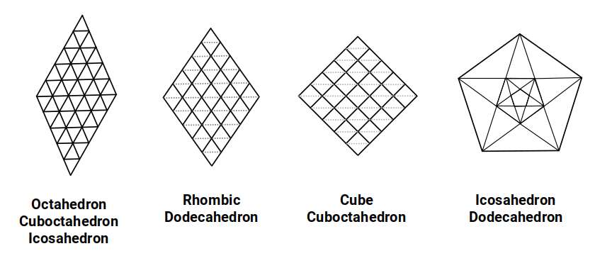
Platonic duals can be compounded so that each side length bisects the other at its midpoint, unifying their mid-spheres. For the icosahedron and dodecahedron, this produces a compound with triangular faces divided into two — the same face found in the 19-point octahedron of fluorine's geonuclear model.

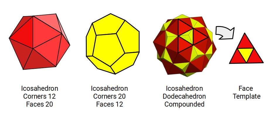
Using the octahedron as a basis, we can map the radii of the jitterbug transformations, adding a dodecahedron compounded with the icosahedron. For each of the four P-orbital sets, this produces the following datasets.

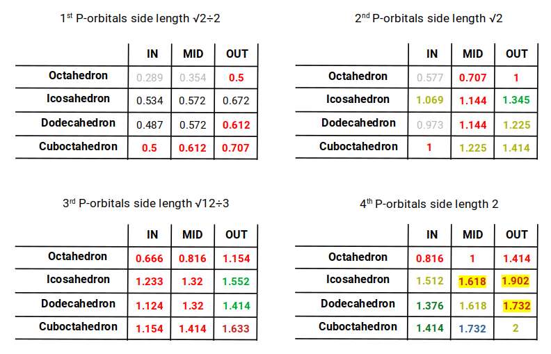
Examining these radii reveals that the out-sphere of the dodecahedron matches the mid-sphere of the cuboctahedron. In the first P-orbital set, this reproduces the radius of oxygen (0.612 Å). In the second set, it gives 1.225 Å — the radius of helium (2). The third set yields 1.414 Å, the approximate radius for D-orbital elements and the fourth P-orbital octahedron. In the fourth dataset, the two polyhedra unify at 1.732 Å, roughly the radius of the F-orbital set.

This compound also reveals the radii of the last three stable P-orbital elements (highlighted in yellow): thallium (81), lead (82), and bismuth (83) — the final stable atoms on the periodic table. Bismuth (83) has a radius of 1.6 Å, which appears in the mid-sphere of the icosahedron–dodecahedron compound and corresponds to the golden ratio. This value defines the two lengths needed to form the pentagonal plane.

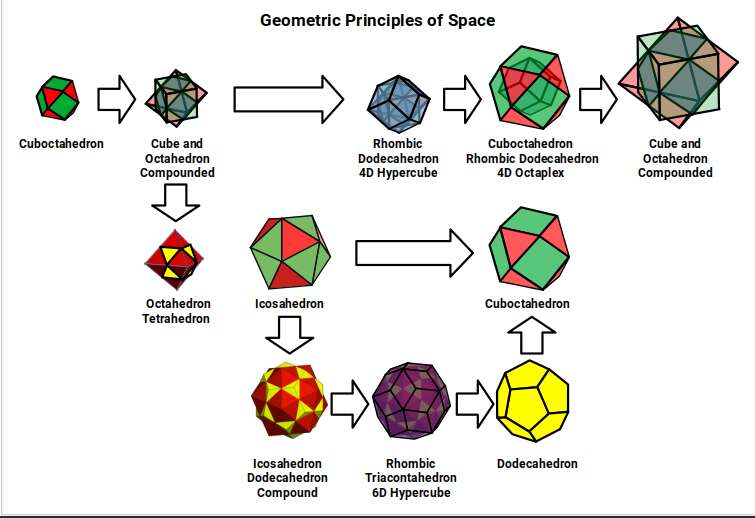
Through our investigation of the P-orbital elements, we have compared the in, mid, and out-spheres of the octahedron, cube, cuboctahedron, rhombic dodecahedron, icosahedron, and dodecahedron. Through the jitterbug transformation the icosahedron is formed, and when compounded with the dodecahedron it defines the mid-sphere of the cuboctahedron.

The rhombic dodecahedron, formed by connecting the corners of a cube–octahedron compound, creates the blueprint for the 4D hypercube. Similarly, connecting the corners of the icosahedron–dodecahedron compound creates the rhombic triacontahedron, which forms the template for the 6D hypercube. This form has 32 corners — which also happens to be the maximum number of electrons that can fill a single shell of the electron cloud.

When the rhombic dodecahedron is nested inside the cuboctahedron, it forms the template for the 4D octaplex. The outer cuboctahedron then provides the foundation for the next cube–octahedron compound. These are the geometric principles through which the initial cuboctahedron doubles in size.

Mapping the in, out, and mid-spheres of these interconnected solids — scaled to the P-orbital octahedra — reveals a striking correlation to experimentally determined values for every element on the periodic table. Each P-orbital is mapped to the out-sphere of the octahedron, which is compounded with the cube at its mid-sphere.

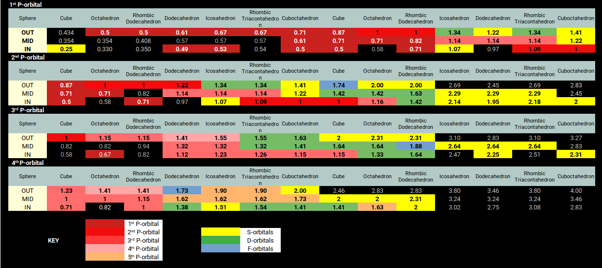
The radii from the first P-orbitals also contain the radii for the preceding S-orbital elements. The second P-orbital dataset overlaps with the D-orbital radii (green) and the lower bound of the F-orbital set, with the radii for another four S-orbitals at the end of the row. The third P-orbital set defines the remaining D-orbital radii and the upper bound of the F-orbitals, followed by two more S-orbital radii. The final set defines the radii for the last pair of S-orbital elements and the three stable elements of the fifth and final P-orbital set, beyond which the radioactive elements begin.

The result is a much closer match to experimental values than the Bohr model. The P-orbital sets tend to level out in radius, while the Bohr model continues to predict a decreasing size. To compensate, the Bohr model predicts a larger S-orbital radius, which brings the P-orbitals into rough alignment but cannot account for the smaller radii of the D and F-orbital sets. The standard explanation attributes this to electron shielding by lower shells — yet for the first P-orbitals, this explanation is untenable. The geometric model is simply the best fit to the experimental data, offering a fresh approach to atomic theory based on geometric ratio.

Conclusion

Current scientific theory treats different aspects of the atom in isolation. The geometric model integrates them, considering the atom as a single entity and providing more accurate predictions of elemental radii than current quantum approaches. Unlike the Bohr model, which breaks down for multi-electron atoms, the geometric model applies across the entire periodic table and addresses some of the most puzzling behaviours of different elements — from why carbon forms hexagonal rings to why nitrogen and oxygen form stable diatomic molecules.

The ability to predict atomic radii through geometric principles has practical implications for materials science, quantum computing, and our understanding of biological processes. This article covers the P-orbital component of the broader framework; for the full picture, explore the Atomic Geometry theory page, along with the companion articles on S-orbital Geometry, D-orbital Geometry (parts 1, 2, 3), The 4D Electron Cloud, The Atom and the Seed of Life, Brillouin Zones, and Geonuclear Physics.

FAQ

How can the electron be a 4D torus?

The electron radius has never been determined — it is best described as a point of charge. In the 4D model, the two circular surfaces of the torus cross paths, defining an x, y, and z axis at a consistent 90° angle (conserving intrinsic angular momentum). When the two surfaces overlap, the internal geometry of a sphere is formed, and any point within it can be identified by defining a point on each circle — explaining measurable point charges. When the circles move apart, the spherical surface disappears, as does the electron. They recombine on the opposite side of the orbital without changing angular momentum, defining a lobe on the opposite side of the torus.

Why has no one proposed a geometric model of the atom before?

Geometry featured prominently in scientific exploration during the Renaissance, but after Newton discovered his law of gravitation, the particle nature of light was adopted. The particle notion of the electron has been maintained even though it displays wavelike properties. When Schrödinger first conceived the S, P, D, and F orbital model, it was based on geometric considerations of the electron cloud, but the insistence on the electron particle introduced quantum probability, obscuring the fact that orbital shapes are real phenomena. Particle physics claims to be the most accurate model of the atom, yet that is only true for hydrogen-like atoms — and because theoretical radii are normally used instead of experimental values, this has never been challenged.

How does P-orbital geometry relate to the rest of Atomic Geometry?

P-orbital geometry is one component of the broader Atomic Geometry framework. The S-orbitals define the foundational spherical structure, the P-orbitals introduce octahedral geometry, the D-orbitals add cubic complexity, and the F-orbitals bring in higher-dimensional forms. Together, the geometric ratios from these nested polyhedra predict the radii of all stable elements — something the Bohr model cannot achieve. For the full picture, see the Atomic Geometry theory page and companion articles on S-orbital geometry and the 4D electron cloud.