The cuboctahedron is arguably the most important of all the Archimedean Solids — the 13 semi-regular polyhedra derived from the Platonic Solids through truncation, expansion, and twisting. With 8 triangular and 6 square faces, it sits at the exact geometric midpoint between the cube and the octahedron. But its significance runs far deeper than geometry. In the hands of Buckminster Fuller it became the Vector Equilibrium — the form of perfect balance, the zero-point from which all other forms arise. In sacred geometry it is the three-dimensional expression of the Flower of Life. And in traditions stretching from ancient India to modern physics, the cuboctahedron keeps appearing wherever nature finds its most balanced state.
Key takeaways
- The cuboctahedron (Vector Equilibrium) is the only polyhedron where all vectors from centre to vertex equal the edge length — a condition of perfect balance that Fuller considered the zero-point form from which all other shapes arise.
- Its 12 vertices define the closest-packed arrangement of spheres — the same twelve-around-one pattern found in metallic crystals, the Seed and Fruit of Life, and the traditional Hindu Akash Kandil.
- In Hindu tradition the Kandil lantern embodies Vishnu the Preserver — the sustainer of cosmic order — its cuboctahedral form a symbol of the force that holds spherical space in equilibrium.
The Vector Equilibrium — Nature's Zero Point
Buckminster Fuller gave the cuboctahedron a new name: the Vector Equilibrium. The reason is a geometric fact unique among all polyhedra: in the cuboctahedron, the distance from the centre to every vertex is exactly equal to the length of every edge. All vectors in the system are equal. No direction is preferred. No vertex is closer to the centre than any other. The result is a form in which all forces and distances are perfectly balanced — geometric equilibrium.
Fuller regarded this as the most fundamental of all three-dimensional forms — the form of zero energy, the condition from which all other forms arise by distortion. In his unified geometry (Synergetics, 1975), he argued that nature's deepest principle is the tendency toward equilibrium — the distribution of energy equally in all directions — and that the cuboctahedron is the purest expression of that principle. Every other three-dimensional form is the Vector Equilibrium under stress: subjected to a force, it transforms into other shapes (through the Jitterbug), but always tends to return to equilibrium when the force is removed.
This idea has deep resonance with modern physics. The quantum vacuum — the ground state of space from which particles emerge — is characterised by zero-point energy: the minimum possible energy a quantum system can hold. If space has the geometric structure that sacred geometry proposes, the form of this minimum-energy state would be precisely the Vector Equilibrium — the shape where all vectors are equal and no direction is favoured. Fuller believed the cuboctahedron was the geometric form of the vacuum's ground state, and that all particles and physical forms arise by displacing the vacuum from this equilibrium.
For the cuboctahedron's mathematical properties, coordinates, and truncation sequence, see the Archimedean Solids chapter in the Guide to Geometry.
Seed of Life and Egg of Life
Both the cuboctahedron and the Seed of Life organise space through the principle of six around one. The Seed is the simplest two-dimensional expression: seven equal circles, one central and six surrounding. The cuboctahedron extends this into three dimensions: twelve spheres around one, the Seed completed into space.
The number progression tells the story: 1 + 6 = 7 (the Seed of Life); 1 + 12 = 13 (the Fruit of Life and the cuboctahedron). Each level of the Flower of Life expansion corresponds to a level of three-dimensional sphere packing, and the cuboctahedron captures the first three-dimensional completion — the moment the flat hexagonal array achieves its full spatial coordination.
The Egg of Life — eight spheres in the arrangement that mirrors the 8-cell stage of embryonic development — is also contained within the cuboctahedron's geometry. The Egg represents the last stage of total completeness before cells begin to specialise, the moment of maximum potential. When all thirteen spheres of the cuboctahedral arrangement are present, they contain the Egg's eight-sphere configuration as a subset. The cuboctahedron adds the further complexity needed to complete the three-dimensional coordination that the Egg begins.
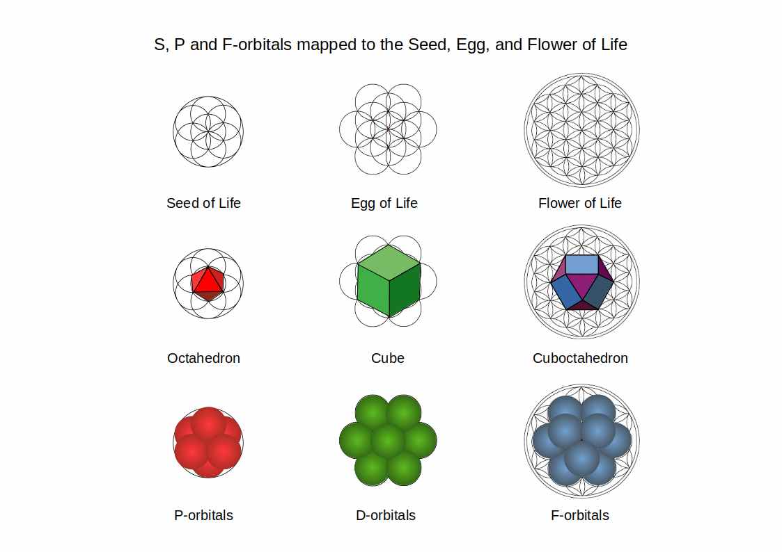
The Cuboctahedron in the Atom
Our Atomic Geometry research proposes that the cuboctahedron is the geometric form of the completed D-orbital electron shell — the Vector Equilibrium's perfect balance expressed at the quantum scale. For the detailed mapping of D-orbitals to the cuboctahedron and its implications for the periodic table, see the Archimedean Solids chapter.
Sphere Packing — Twelve Around One
Place a sphere on a table and surround it with identical spheres, each touching the central one. How many fit? In two dimensions, the answer is six — the same six-around-one pattern as the Seed of Life. In three dimensions the answer is twelve, and the centres of those twelve surrounding spheres sit at the vertices of a cuboctahedron. Toggle the Spheres layer in the interactive above to see this arrangement.
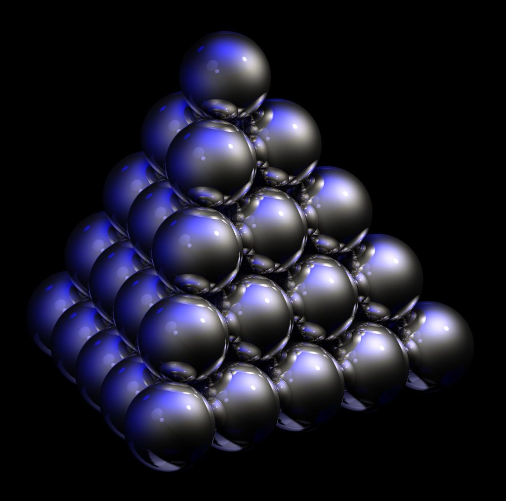
The equal-vector property of the Vector Equilibrium is what makes this arrangement inevitable. When spheres pack as tightly as possible, they naturally arrive at the form where all distances are equal — the cuboctahedron. Nature doesn't calculate this; it simply finds equilibrium, and the cuboctahedron is what equilibrium looks like in three dimensions. For the mathematical details — FCC lattice, Kepler's conjecture, and the proof by Thomas Hales — see the Archimedean Solids chapter.
Vishnu's Lantern — The Cuboctahedron in Hindu Tradition
The cuboctahedron's form appears in one of the most recognisable objects in Hindu culture: the Akash Kandil (or simply Kandeel) — a hanging lantern displayed during Diwali. Its diamond-shaped form, with panels radiating equally from a central point, mirrors the geometry of the cuboctahedron — light extending in all directions from a single source.
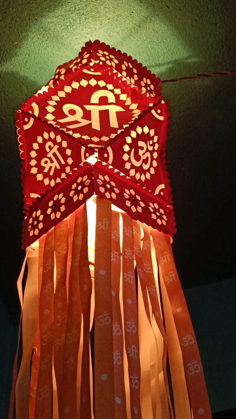
The Kandeel is sacred to Vishnu — the Preserver, the sustainer of cosmic order. In the Hindu Trimurti, Brahma creates and Shiva destroys, but Vishnu is the force that holds the cosmos in balance between creation and dissolution. This is precisely the role of the cuboctahedron: just as the Vector Equilibrium sustains spherical space — holding twelve spheres in perfect balance around a centre — Vishnu sustains the cosmic order, preserving the equilibrium from which all forms arise and to which they return.
The Star of Lakshmi — an eight-pointed star sacred to Vishnu's consort — expresses the same principle: equal extension in all directions, perfect symmetry, cosmic balance. The Diwali festival itself celebrates the triumph of light over darkness, knowledge over ignorance — and the Kandeel, glowing at its centre and radiating outward in cuboctahedral symmetry, is a physical embodiment of Vishnu's sustaining light holding space in equilibrium.
In the next chapter, we explore The Torus — the doughnut-shaped form of flow and return that appears everywhere from apple cores to magnetic fields.
FAQ
What is special about the cuboctahedron compared to other polyhedra?
The cuboctahedron is the only polyhedron in which the distance from the centre to every vertex equals the edge length — all vectors are equal. Buckminster Fuller named it the Vector Equilibrium for this reason, considering it the form of zero energy and perfect geometric balance from which all other forms arise by distortion.
How does the cuboctahedron relate to the Flower of Life?
The cuboctahedron is the 3D realisation of the Fruit of Life (13 circles within the Flower of Life). Its 12 vertices correspond to the 12 outer circle centres of the Fruit projected into 3D space. Its hexagonal cross-section matches the hexagonal structure of the Flower of Life. The same six-around-one principle organises both forms.
What is the Jitterbug transformation?
Discovered by Buckminster Fuller, the Jitterbug is a continuous transformation in which a flexible cuboctahedron model collapses through the icosahedron to the octahedron to a flat plane. It demonstrates that these forms are not separate objects but stages of a single dynamic process — related by continuous physical transformation rather than static geometric similarity.
Why is the cuboctahedron important in atomic structure?
In metallic crystals (copper, gold, aluminium), each atom is surrounded by 12 nearest neighbours arranged at the vertices of a cuboctahedron — the face-centred cubic (FCC) lattice. Our Atomic Geometry proposes that the cuboctahedron specifically describes the completion of the D-orbital electron shell, with the Vector Equilibrium's zero-point character explaining the unusual stability of elements like zinc.