Introduction
Infinity is usually thought of as something impossibly large — a number that never ends. But mathematicians have known for over 150 years that infinity comes in different sizes, and that some infinities are strictly larger than others. More surprisingly, the familiar whole numbers (1, 2, 3…) and the decimal numbers (0.1, 0.25, 3.14159…) represent two different sizes of infinity that cannot be directly compared using standard mathematics.
This article presents a new approach from Geometric Maths — a framework built on the principles of Euclidean geometry extended into higher dimensions. The central claim is striking: by viewing numbers not as points on a one-dimensional line, but as structures occupying two, three, and even four dimensions, the longstanding puzzles of infinity become solvable. The famous Continuum Hypothesis — one of the great open problems in mathematics — yields to this geometric treatment.
Why does this matter?
The mathematics of infinity is not merely abstract. It underpins the logical foundations on which all of modern mathematics rests. Unsolved problems in this area — the Continuum Hypothesis, the Russell Paradox, the Riemann Hypothesis — represent genuine gaps in our understanding of number. A coherent resolution would reframe how mathematics itself is structured, with consequences reaching into physics, computation, and our understanding of reality.
The Challenge of Infinity
Counting may appear to be among the most elementary of mathematical operations. Yet the nineteenth-century mathematician Georg Cantor demonstrated, through his now-famous diagonal proof, that it is impossible to enumerate all numbers.
The argument is elegant. Suppose you try to write a complete list of every number. Cantor showed that you can always construct a new number not on your list: take the first digit of the first entry, the second digit of the second entry, and so on — then change each digit. This new number cannot appear anywhere on your list, because it differs from every entry in at least one position. Therefore, no list can ever be complete.
The situation becomes more complex when the real numbers — every possible decimal, rational and irrational — are included. If the infinite set of whole numbers (written ℵ0, pronounced "aleph-zero" — Cantor's notation for the smallest type of infinity) cannot be listed, how can the real numbers (ℵ1, the next size of infinity, encompassing all decimals)?
Cantor proved that ℵ1 is strictly denser than ℵ0 — there are more decimal numbers than whole numbers — but could not determine by exactly how much. The Continuum Hypothesis arose from precisely this question: is there an infinity sitting between ℵ0 and ℵ1, or do they sit directly adjacent to one another? It has remained one of the great open questions at the heart of number theory for over a century.
The Size of Infinity
The first problem is measuring the size of infinity. What we can establish is this: if an infinite set is missing some numbers, it has lower density than another. Through bijection — a technique that pairs up elements from two sets in a one-to-one correspondence, like matching every left shoe to a right shoe — we can compare the sizes of infinite sets without directly counting them. This is how we know ℵ1 has greater density than ℵ0: there are more decimal fractions than whole numbers, even though both sets are infinite.
Since infinity is commonly treated as boundless, the only available tools have been those that project the outcome of a relationship into infinity. Without knowing the size, it is impossible to determine how much larger one type of infinity is than another. A new framework is required — one that allows us to qualify ℵ1, ℵ0, and any other type of infinity. If an infinite set can be found sitting between them, the Continuum Hypothesis will be solved.
Law of Equivalence
The Law of Equivalence states that if two quantities are halves of the same thing, they are equal to one another. In Geometric Maths, this principle is derived directly from Euclid's axioms:
(7) Things which are halves of the same things are equal to one another.
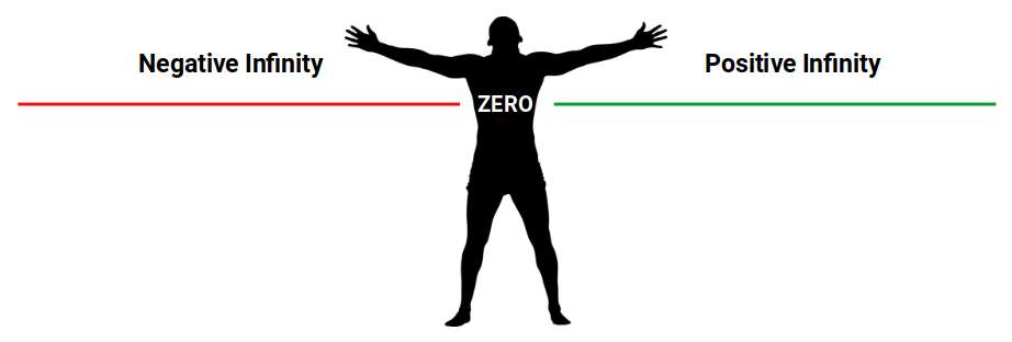
If we halve infinity, we obtain two equivalent infinities. The clearest example on the number line is the infinite set of positive numbers and the infinite set of negative numbers — each a perfect mirror of the other, with zero at the centre.
Non-Polar Numbers
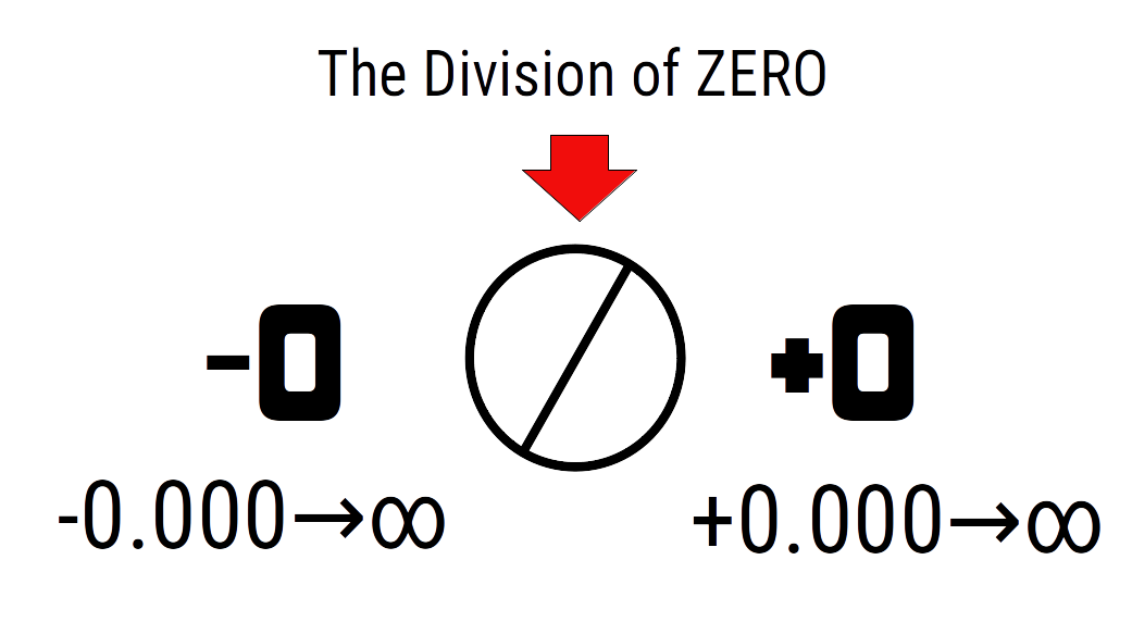
Zero presents certain difficulties in mathematics. Whether it belongs to the set of whole numbers is often treated as a matter of convention. It does not exhibit polarity the way other numbers do, and any calculation involving zero tends to produce zero. That is the consequence of its non-polarity.
To complete the set of whole numbers (ℵ0), Geometric Maths introduces a distinction that has been conventionally overlooked: zero⁺ and zero⁻. All numbers in reciprocal space — the fractional numbers between zero and one, such as 0.5 or 0.333…, which are the "flipped" versions of the whole numbers (½ is the reciprocal of 2, ⅓ the reciprocal of 3) — begin with +0.xxx…, and the same holds for negative numbers, expressed as −0.xxx…
With the addition of +0 and −0, the full number range becomes:
−∞ ← −3, −2, −1, −0, 0, +0, +1, +2, +3 → +∞
Due to its non-polarity, zero may be optionally removed so that positive and negative number space forms a one-to-one bijection. We define ℵ0 as the whole numbers from zero to infinity:
0, 1, 2, 3 → ∞ = ℵ0
Any number outside this set — that is, all decimal fractions that are not whole numbers — is categorised as part of ℵ1. This categorisation provides the framework within which the Continuum Hypothesis will be addressed.
Uncountability
Cantor's diagonal proof demonstrated that numbers cannot be fully listed. But does that mean they cannot be counted? There is an important distinction: making a list creates a record, whereas counting performs a calculation.
In its simplest terms, counting sequential numbers begins at zero and adds one repeatedly — an infinite loop that generates the entire set. Performing a calculation is distinct from writing down the result; the result only exists once the calculation is complete.
In the case of infinity, there are numbers that exhibit infinite decimal expansions — √2 is a familiar example. We know how it is constructed, yet we have never been able to write it in full, because it is an infinite decimal fraction. In this sense, no number can ever be fully listed; it can only be calculated to a given degree of precision.
Number Systems
To understand counting more precisely, we return to fundamentals. Our standard number system is written in base 10 — meaning we use ten symbols (0 through 9), and once we have used all of them, we start a new column. That is why after 9 we write 10, and after 99 we write 100. When a number is formulated, a base system creates a grid of a specific dimension.
The standard number grid as first taught looks like this:
1 2 3 4 5 6 7 8 9 10
11 12 13 14 15 16 17 18 19 20
21 22 23 24 25 26 27 28 29 30
31 32 33 34 35 36 37 38 39 40
41 42 43 44 45 46 47 48 49 50
51 52 53 54 55 56 57 58 59 60
61 62 63 64 65 66 67 68 69 70
71 72 73 74 75 76 77 78 79 80
81 82 83 84 85 86 87 88 89 90
91 92 93 94 95 96 97 98 99 100
Remember Zero
This grid is the one introduced when multiplication is first taught. In the x direction (→), numbers repeat from 1 through 9, then a double-digit number appears — 10 — which has a zero in its second position. Examining this table, we notice the symmetry is off. We can begin to correct it by adding a zero to the top row, so the numbers run from 01 to 10 in the x direction:
01 02 03 04 05 06 07 08 09 10
11 12 13 14 15 16 17 18 19 20
21 22 23 24 25 26 27 28 29 30
31 32 33 34 35 36 37 38 39 40
41 42 43 44 45 46 47 48 49 50
51 52 53 54 55 56 57 58 59 60
61 62 63 64 65 66 67 68 69 70
71 72 73 74 75 76 77 78 79 80
81 82 83 84 85 86 87 88 89 90
91 92 93 94 95 96 97 98 99 100
Number Order
To complete the defined set for ℵ0, zero must be included at the start. Once placed, all numbers align correctly. The first digits proceed in both x and y directions from 0 to 9, consistent with our definition of ℵ0.
This symmetry is significant: the 10 times table runs along the y-axis, the 11 times table runs along the diagonal from 00 to 99, and the 9 times table appears on the second diagonal. The 1× table runs through the sequential rows — the simplest to calculate — and creates the sequence of numbers structured into mathematical order using a base system.
There is, however, a small problem. As numbers grow larger, more digits are required to accommodate their position. A grid of 100 squares contains only 99 of the numbers; the number 100 begins a new row, introducing triple digits for the first time:
00 01 02 03 04 05 06 07 08 09
10 11 12 13 14 15 16 17 18 19
20 21 22 23 24 25 26 27 28 29
30 31 32 33 34 35 36 37 38 39
40 41 42 43 44 45 46 47 48 49
50 51 52 53 54 55 56 57 58 59
60 61 62 63 64 65 66 67 68 69
70 71 72 73 74 75 76 77 78 79
80 81 82 83 84 85 86 87 88 89
90 91 92 93 94 95 96 97 98 99
100
Examining the diagonals, any square diagonal to another will either add or subtract 9 or 11 from its total. Multiplication is a specific form of addition expressed only along the diagonals of the base 10 number grid.
Zero as Placeholder
As sequential numbers progress, additional zeros are required to distinguish each number from the others. In the first row we have single-digit numbers. The next nine rows comprise double-digit numbers. As a third digit is introduced, the number of possibilities increases dramatically. This logarithmic expansion occurs at different rates depending on the base system used.
The expansion of numbers is a direct consequence of zero as a placeholder for larger values. We append zero to the end of the number and begin again, incrementing each unit at each step:
0000 0001 → 0009
0010 0011 → 0099
0100 0101 → 0999
1000 1001 → 9999
The numbers 01, 001, and 0001 are extensions of this concept — each leading zero brings a number into context with the next larger set. With four digits, numbers run from 0000 to 9999. Therefore, there are an infinite number of zeros preceding any given number; we simply omit them for convenience.
Infinite Numbers
The key to counting is our ability to extrapolate from the infinite. We do not write 001 every time we perform a calculation; the surplus zeros are removed without issue. However, when dealing with infinite sets, we must account for the infinite even if we cannot write it down.
Logic tells us that if numbers are infinite, so is the number of digits required to express them. The number one appears as a single digit — yet 01 and 001 are equally valid expressions. When considering the infinite, there is no reason to limit the zeros placed in front of a number.
By placing an infinite number of zeros in front of each number, the number grid takes on a different quality — one that allows us to explore the infinite side of numbers. In the notation below, ∞0 represents an infinite number of leading zeros, and the part after the arrow is what differs within the set:
∞0→0 ∞0→1 → ∞0→9
∞0→10 ∞0→11 → ∞0→99
∞0→100 ∞0→101 → ∞0→999
∞0→1000 ∞0→1001 → ∞0→9999
Notice that on the right-hand side another pattern emerges — all numbers are composed of the digit nine. In base 10, 9 is the final digit, and following this logic all numbers form an infinite set of nines at the point of infinity:
∞ → 99999 → ∞
This result is a consequence of base 10. Under a different base system, the terminal digits will differ. To uncover the deeper mystery of infinity, we must find a way to transcend this limitation.
Base Infinity
A base number system is simply the set of symbols — or digits — we use to write numbers. Our everyday system uses ten symbols (0 through 9), which is why it is called base 10. Different base systems operate throughout daily life: time is measured partly in base 12 (the number 12 being equivalent to zero at midnight, hence the word "o'clock"); computers use binary (base 2: only 0 and 1) and hexadecimal (base 16) in everyday operations.
The simplest system is binary — an on/off, zero/one mechanism, the minimum required to process any calculation. Base 1 would express only a single digit and therefore display only zero.
The Sumerians used a base 60 system for their calendars. When considering infinity, we must also ask: how many base systems are there? The answer is that there are an infinite number of base systems:
- base 1 = 00000000
- base 2 = 010100101
- base 3 = 012020121
As the base number increases, so does the number of options available for a single digit, approaching infinity. At base infinity, each digit could be any symbol from the infinite line of already existing numbers:
base ∞ = ∞…∞∞∞…∞
Wholes and Fractions
In base ∞, another property of numbers helps clarify: the decimal fraction. All numbers can be expressed as a decimal fraction. For whole numbers, the fractional part is denoted by an infinite number of zeros — just as we omit leading zeros at the start, the same applies to zeros appended to the fractional part. When viewed with the infinite fraction expressed:
0 = ∞→…000.000→…∞ 1 = ∞→…001.000→…∞ 2 = ∞→…002.000→…∞
The decimal point divides whole from fractional space, just as zero divides positive from negative number space.
Whole numbers can therefore be defined as numbers that exhibit an infinite number of zeros after the decimal point — even in base infinity:
A whole number in base infinity: ∞→…∞∞∞.000→…∞
If we invert this — placing the infinite set of zeros on the left and the infinite set of infinities on the right — we obtain the infinite set of reciprocal numbers between zero and one (the "flipped" fractions such as ½, ⅓, ¼):
A reciprocal number in base infinity: ∞→…000.∞∞∞→…∞
In Geometric Maths, reciprocal numbers are categorised as a distinct class — one of the mechanisms by which the Russell Paradox is resolved.
The Decimal Point
When viewed in their full decimal format, numbers are formed from two sets of infinity — the whole part and the fractional part — separated by a decimal point. Including the negative numbers, the pattern becomes clear:
∞… ← −1.0 | −0.0 | 0 | +0.0 | +1.0 → …∞
The decimal point divides whole and fractional space in the same way that zero divides positive and negative number space — it is a boundary that holds no identifying characteristic of its own.
Using bijection, we can confirm that the positive and negative portions of the number line are in perfect correspondence, consistent with the Law of Equivalence: infinity divides into two equivalent parts. The same holds for each infinity either side of the decimal point. Whatever can be constructed on one side can also be constructed on the other. As whole numbers form the foundation for ℵ0 and fractions the basis for ℵ1, these observations bring us close to the final picture needed to answer the Continuum Hypothesis.
Uniqueness
When expressed in base infinity, each unit of a number has a unique expression that completely differentiates it from all others. In base infinity, this uniqueness is expressed as a single digit which, by its nature, differs from all others. In this way, we can "collapse" the entire list of infinite whole numbers into a single infinity:
Infinite potential:
∞ ∞ ∞ →…∞
↓ ↓ ↓ ↓ ↓ ↓ ↓ ↓ ↓
Unique expression:
+1 +1 +1 →…∞ = ∞
Once a number is written down, it forms a unique expression and no further digits are required to represent it. This is analogous to the scientific notion of observation: a number written down is an observable phenomenon. Any symbol can be assigned to any number in existence, but once it represents a particular quantity, it must be removed from the infinite set.
As each unique number is added into infinity, we are summing an infinite series of +1 — which is precisely how the whole number series is formed:
0 + 1 = 1
1 + 1 = 2
2 + 1 = 3
By adding 1 at each stage, the infinite set of sequential whole numbers is produced. This lies at the heart of the infinity equation:
0 ±1 = ±∞
This is a recursive calculation that at each step generates the next whole number. Numbers are not written — they are calculated. Reiterated into infinity, the result reaches one end of the whole number line depending on the ratio of +1s to −1s. More fundamentally, it suggests that the infinite set of whole numbers is derived from the notion of ±1, since for any number imaginable there is always one less and one greater.
Solving the Infinite
With the foundations established, we can now construct the framework that resolves the Continuum Hypothesis.
Through the observation that in base infinity the whole number set "collapses" into a single infinity, we have avoided the pitfalls of the listed number set. Instead of trying to enumerate numbers (which Cantor proved impossible), we address uncountability through a new methodology — observing how we extrapolate from an infinite set only those digits that form a particular number. Since an infinite set can be represented as a single unique digit, the diagonal argument is sidestepped entirely, and the infinite series collapses into a single infinity.
As the fractional side of a whole number must equal an infinite set of zeros, we can determine:
ℵ0 = ∞
The solution to ℵ0 is determined through observations in base ∞.
We know the two infinities — whole and fractional — are equivalent because they exhibit a one-to-one correspondence. We can therefore collapse the fractional side into a single infinity as well. The result is an infinity followed by a decimal fraction also denoted by infinity:
∞.∞
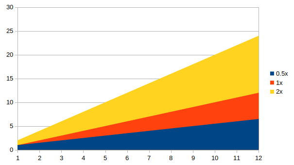
Infinite Proportions
Order is a critical concept when dealing with infinity. Just as a computer must execute lines of code in a specific sequence to run a programme, so too must the order of mathematical operations be preserved when dealing with the infinite.
When considering decimal fractions, the number before the decimal point represents a whole number — and we have established that this collapses into a single infinity: ℵ0 = ∞. Each whole number is, however, accompanied by an infinite potential fraction:
0.∞, 1.∞, 3.∞ → ∞
If for every whole number there is an infinite fraction, the ratio between the two parts is:
1 : ∞
It follows that if ℵ0 = ∞, then ℵ1 = ∞².
ℵ0 = ∞, therefore ℵ1 = ∞²
ℵ0 has a proportional relationship to ℵ1 that is a square power. ∞² is more formally defined in our concept of 4D Squaring. As far as we are aware, this is the first explicit definition mathematics has produced for these two identities. Having established the ratio between them, we now have all the elements required to solve the Continuum Hypothesis.
Overcoming the Paradox
One might assume the Continuum Hypothesis is now solved: if infinities are always equivalent and equal, it is only by the order of their appearance that a difference can be found.
In fact, precisely this difference between whole and fractional infinities is where the logical construct encounters its first difficulty — and this problem lies at the heart of the Russell Paradox.
The Russell Paradox identifies a small but highly significant point: all whole numbers above one have a reciprocal value in the space between 0 and 1. The number 1 does not have a reciprocal value in that space. If zero were excluded from ℵ0, the space between 0 and 1 would not be accounted for. Since reciprocal values are defined as the inverse of whole numbers greater than one, they all fall within this unit space — yet none of these reciprocals are themselves whole numbers.
The paradox becomes visible: if the whole numbers appear as reciprocals in the space between zero and one, and no such reciprocals appear in the space between 1 and 2, should there not be more numbers in reciprocal space than in other number spaces?
And yet we have asserted that ℵ1 = ∞² based on the equivalence of all infinities for each integer. Resolving this tension requires careful logic — approaching infinity from the wrong angle makes it very easy to become lost in such logical loops.
Reciprocal Space
Our enquiry has led us to the identity ∞.∞ as the basis for the relationship between ℵ0 and ℵ1, with each infinite set equivalent at this stage. We have included zero in both sets, giving the identity 0.0 within the set.
When the fractional part of a number comprises only zeros, it is a whole number. When the whole part consists only of zeros, the number is a reciprocal. We therefore have two types of number — whole and reciprocal — represented by the same qualities exhibited by both infinite sets.

Examining the fractional side: since whole numbers appear only when the fractional number equals zero, one unit must be removed from the infinite series for each whole number. The ratio between whole and fractional infinite sets established thus far is 1:∞. Subtracting 1 from the fractional side to account for the zero that forms each whole number gives:
1 : ∞−1
Examining the whole number side: whenever it equals zero, a reciprocal number is created. As reciprocal values represent one out of the infinite set of wholes, one must also be subtracted from this side:
∞−1 : ∞−1²
Note that since there are an infinite number of fractions between each number space, the fractional set is squared. This arises from the order of appearance, not from the magnitude of the infinite, which remains in equilibrium throughout.
This gives us three categories of number: Whole, Reciprocal, and Fractions greater than one.
The Final Solution
The Power of Infinity
With these three categories established, we have all the elements required to formulate the solution to the Continuum Hypothesis. The identities of the three number types are:
- Whole: ∞−1
- Fractional: (∞−1)²
- Reciprocal: (∞−1) × (∞²−1)
The reciprocal values contain both whole and fractional infinite sets, giving the reciprocal set an identity of:
Reciprocal: ∞−1³
The full comparison is therefore:
- Whole: ∞−1
- Fractional: (∞−1)²
- Reciprocal: (∞−1)³
Each set appears with the same identity, increasing through powers. To put this plainly: raising a number to a power means multiplying it by itself that many times — x² means x×x (a square), x³ means x×x×x (a cube). In Geometric Maths, powers are functions — not numbers — and are responsible for the transformation of dimension: from a one-dimensional line into the second dimension, and then into the third and beyond.
The conclusion is that numerical space is not a one-dimensional construct. Attempting to classify numbers without consideration of the geometry of the number line is therefore impossible. This becomes clearer when numbers are explored from a higher-dimensional perspective.
Number Geometry
It is generally agreed that x² demonstrates the formation of a square, and x³ that of a cube. Euclid clearly stated that "the edges of a surface are lines" — a proposition never shown to be false within Euclidean geometry. Geometric Maths is founded on these Euclidean laws, avoiding unnecessary complication.
Consider the relationship between the whole numbers and the fractional set. Whereas the wholes contain one infinity, the fractional set is squared. We represent this by introducing a second axis at 90° to the first, labelling one axis Whole and the other Fractional.
The reciprocal values between zero and one are absent from this set, comprising their own reciprocal space. Marking out this region gives the following result:
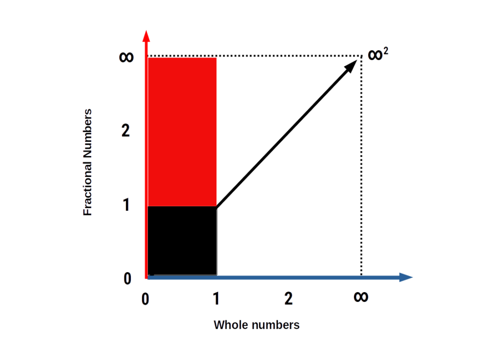
Those familiar with mathematics may begin to see from this image how a direct solution to the Riemann Hypothesis can be formulated — the next significant challenge on the list of unsolved mathematical problems.
3D Number Space
With the 2D infinite number plane established, we must now accommodate the reciprocal numbers. These contain both all whole numbers and all fractions above one. The derived identity for the reciprocal shows that it is raised to the power of 3.
Adding another axis at 90° to the square plane forms an x, y, z coordinate system — a cube with a specific portion removed:
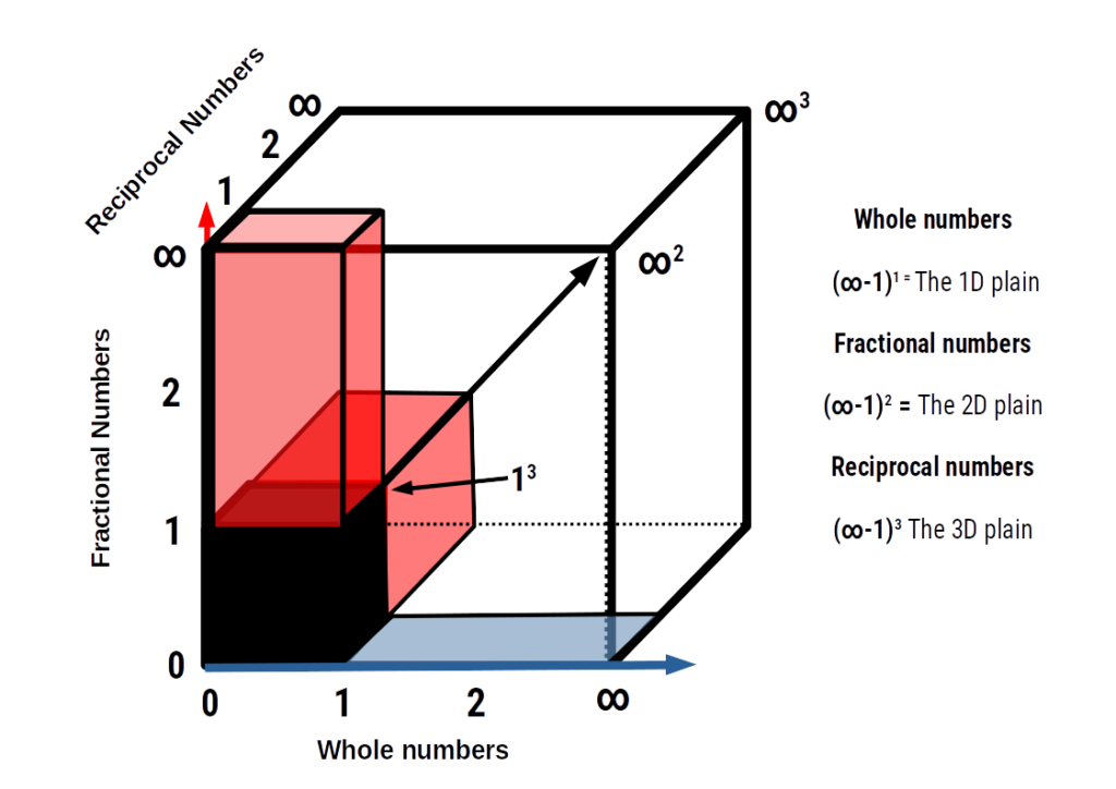
It is worth noting that the three types of infinite number set each inhabit a specific geometric dimension. A line is not merely the side of a 2D shape — it is the 2D plane viewed edge-on, rotated in 3D space. The 2D plane is itself composed of an infinite set of lines projected in the y-direction. At any point on the surface of the square, two lines oriented at 90° intersect, representing a combination of two infinite sets: whole numbers forming the line, and the surface of the square generated by the infinite fraction.
Similarly, it is the volume of the cube that contains all reciprocal values — a combination of both whole and fractional numbers into one infinity. Just as any point within the square can be selected, the same applies within the cube. Each such "number point" is a composition of the three types of infinite set. It is their combination within 3D space that gives each number its mathematical context. Each type of infinity can be expressed on the number line — just as 1, 1², and 1³ all appear in the same place yet are entirely distinct. Only from a higher-dimensional perspective can the complete picture be seen.
4D Number Space
The model of the infinite number cube presents several peculiarities worth further investigation.
The nature of the number one creates a specific boundary we call the Infinity of ONE. This boundary becomes easier to identify when placed inside the cube. The volume of a cube is a mathematically determined quantity. We can specify the dimensions of the base cube of 1, which holds the reciprocal characteristics of all numbers. All whole and fractional numbers exist in the space above one, occupying the cubic space in the far upper corner. Since reciprocal space has a one-to-one correspondence to the combined set of whole and fractional numbers above one, they must be of equivalent density. If the size of reciprocal space is 1³, the same must hold for the cube containing all whole and fractional numbers combined — producing two cubes at opposite corners:
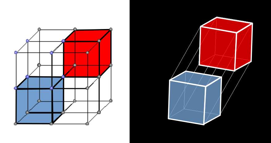
The result is a numerical model that takes the form of a 4D hypercube. When rotated on its w-axis, the two cubes swap positions. The entire set of decimals above one, found in the space of the red cube, is extracted from the reciprocal number space (blue cube) between zero and one.
The 4D Perspective
What has been revealed thus far represents only one eighth of the complete picture presented by Geometric Maths. The 4th Dimensional Number Cube exhibits eight types of reciprocal space compared to our traditional notion of numbers. Each is reflected into eight whole number corner cubes, all of the same spatial dimension.
This leads to a new hypothesis for a universal theory — one that examines the nature of reality from the micro to the macro as exhibiting the qualitative aspects of high-dimensional solids. Objects in the fourth dimension or higher cannot be measured and are therefore imperceptible to standard scientific investigation. However, a mathematics founded on the laws of geometry can account for many of the as yet unanswered questions that confound current research.
Conclusion
The dilemmas posed by infinity — which traditional mathematics, limited to the complex plane, cannot resolve — become tractable when numbers are placed into a higher-dimensional geometric space.
The key results of this investigation are:
- ℵ0 = ∞ and ℵ1 = ∞²: the first explicit quantified relationship between the two sizes of infinity that appear in the Continuum Hypothesis.
- Whole numbers, reciprocal numbers, and fractions above one are three geometrically distinct categories, each occupying a different dimension — line, plane, and volume respectively.
- The Russell Paradox is resolved by recognising that reciprocal space forms its own category, separate from both whole and fractional number spaces.
- The resulting structure takes the form of a 4D hypercube, revealing seven additional number spaces with no definition under current mathematical axioms.
Where traditional mathematics has treated numbers as points on a line, Geometric Maths treats them as structures with dimensional depth. The infinite, far from being a formless expanse, has a precise geometric architecture. Understanding this architecture does not merely solve long-standing abstract puzzles — it reframes how we think about number, dimension, and ultimately the structure of reality itself.
FAQ
How can numbers exist in a higher number space?
A line is a one-dimensional structure. When the line is rotated, it produces the cross — see our article on Zero². This transforms the line into a 2D plane. Similar processes transform the 2D plane into an x, y, z axis system, mapped on the hexagonal number plane.
How does folding or reflecting number space solve infinity?
We propose that the infinite set of whole numbers is contained within a numerical space of the same dimension as the reciprocals. This sees all real numbers above one reflected into the space between zero and one, identifying the unique relationship between these two number regions and square and root operations. For further reading, see our articles on the Infinity of ONE and the ZERO boundary.
What is the Continuum Hypothesis in plain English?
We know there are different sizes of infinity. The smallest countable infinity (whole numbers, called ℵ0) is smaller than the infinity of all decimal numbers (ℵ1). The Continuum Hypothesis asks: is there a size of infinity sitting between these two, or do they sit directly next to each other? This has remained unsolved since Cantor posed it in the 1870s.
What is the Russell Paradox and why does it matter here?
The Russell Paradox identifies a logical contradiction in set theory: all whole numbers above 1 have a reciprocal value in the space between 0 and 1, yet none of those reciprocals are themselves whole numbers. This creates an apparent asymmetry between number regions. Geometric Maths resolves it by treating whole numbers, reciprocals, and fractions above one as three distinct categories, each occupying its own geometric dimension.